4.18. Chapter 4 Spectroscopy#
4.19. Analyze Spectrum#
![]()
part of
MSE672: Introduction to Transmission Electron Microscopy
Spring 2024
| Gerd Duscher | Khalid Hattar |
| Microscopy Facilities | Tennessee Ion Beam Materials Laboratory |
| Materials Science & Engineering | Nuclear Engineering |
| Institute of Advanced Materials & Manufacturing | |
Background and methods to analysis and quantification of data acquired with transmission electron microscopes.
4.19.1. Load relevant python packages#
4.19.1.1. Check Installed Packages#
import sys
import importlib.metadata
def test_package(package_name):
    """Test if package exists and returns version or -1"""
    try:
        version = importlib.metadata.version(package_name)
    except importlib.metadata.PackageNotFoundError:
        version = '-1'
    return version

if test_package('pyTEMlib') < '0.2024.2.3':
    print('installing pyTEMlib')
    !{sys.executable} -m pip install  --upgrade pyTEMlib -q

print('done')
installing pyTEMlib
done
4.19.2. First we import the essential libraries#
All we need here should come with the annaconda or any other package
The xml library will enable us to read the Bruker file.
%matplotlib widget
import matplotlib.pyplot as plt
import numpy as np
import sys
import os
if 'google.colab' in sys.modules:
    from google.colab import output
    from google.colab import drive
    output.enable_custom_widget_manager()


import xml.etree.ElementTree as ET
from scipy.ndimage import gaussian_filter

import pyTEMlib
# import pyTEMlib.viz as plot
import pyTEMlib.file_tools as ft
import pyTEMlib.eds_tools as eds

# For archiving reasons it is a good idea to print the version numbers out at this point
print('pyTEM version: ',pyTEMlib.__version__)
pyTEM version: 0.2024.02.2
4.19.3. Select File#
Please note that the above code cell has to be finished before you can open the * open file* dialog.
Test data are in the SEM_example_data folder, plese select EDS.rto file.
datasets = ft.open_file()

chooser = ft.ChooseDataset(datasets)
dataset = chooser.dataset
dataset.plot()
4.19.3.1. Function to read Bruker files#
The data and metadata will be in a python dictionary called tags.
import codecs

def open_Bruker(fname):
    tree = ET.parse(fname)
    root = tree.getroot()
    spectrum_number = 0
    i=0
    image_count = 0
    o_count = 0
    tags = {}
    for neighbor in root.iter():
        #print(neighbor.attrib.keys())
        if 'Type' in neighbor.attrib:
            if 'verlay3' in neighbor.attrib['Type'] :
                semImage = neighbor
                #print(neighbor.attrib['Type'])
                if 'Name' in neighbor.attrib:
                    print('\t',neighbor)
                    print('\t',neighbor.attrib['Type'])
                    print('\t',neighbor.attrib['Name'])
                    print('\t',neighbor.find("./ClassInstance[@Type='TRTSpectrumList']"))
            #if 'TRTImageOverlay' in neighbor.attrib['Type'] :
            if 'TRTCrossOverlayElement'in neighbor.attrib['Type'] :
                if 'Spectrum' in neighbor.attrib['Name']:
                    #print(o_count)
                    o_count+=1
                    if 'overlay' not in tags:
                        tags['overlay']= {}
                    if 'image'+str(image_count) not in tags['overlay']:
                        tags['overlay']['image'+str(image_count)] ={}
                    tags['overlay']['image'+str(image_count)][neighbor.attrib['Name']] ={}

                    over = tags['overlay']['image'+str(image_count)][neighbor.attrib['Name']]


                    for child in neighbor.iter():
                        if 'verlay' in child.tag:
                            #print(child.tag)
                            pos = child.find('./Pos')
                            if pos != None:
                                over['posX'] = int(pos.find('./PosX').text)
                                over['posY'] = int(pos.find('./PosY').text)
                #dd = neighbor.find('Top')
                #print('dd',dd)
                #print(neighbor.attrib)
            if 'TRTImageData' in neighbor.attrib['Type'] :
                #print('found image ', image_count)
                dd = neighbor.find("./ClassInstance[@Type='TRTCrossOverlayElement']")
                if dd != None:
                    print('found in image')
                image = neighbor
                if 'image' not in tags:
                    tags['image']={}
                tags['image'][str(image_count)]={}
                im = tags['image'][str(image_count)]
                im['width'] = int(image.find('./Width').text)  # in pixels
                im['height'] = int(image.find('./Height').text)  # in pixels
                im['dtype'] = 'u' + image.find('./ItemSize').text  # in bytes ('u1','u2','u4')
                im['plane_count'] = int(image.find('./PlaneCount').text)
                im['data'] = {}
                for j in range( im['plane_count']):
                    #print(i)

                    img = image.find("./Plane" + str(i))
                    raw = codecs.decode((img.find('./Data').text).encode('ascii'),'base64')
                    array1 = np.frombuffer(raw, dtype= im['dtype'])
                    #print(array1.shape)
                    im['data'][str(j)]= np.reshape(array1,(im['height'], im['width']))
                image_count +=1
            if 'TRTDetectorHeader' == neighbor.attrib['Type'] :
                detector = neighbor
                tags['detector'] ={}
                for child in detector:
                    if child.tag == "WindowLayers":
                        tags['detector']['window']={}
                        for child2 in child:
                            tags['detector']['window'][child2.tag]={}
                            tags['detector']['window'][child2.tag]['Z'] = child2.attrib["Atom"]
                            tags['detector']['window'][child2.tag]['thickness'] = float(child2.attrib["Thickness"])*1e-5  # stupid units
                            if 'RelativeArea' in child2.attrib:
                                tags['detector']['window'][child2.tag]['relative_area'] = float(child2.attrib["RelativeArea"])
                            print(child2.tag,child2.attrib)

                    else:
                        #print(child.tag , child.text)
                        if child.tag != 'ResponseFunction':
                            if child.text !=None:
                                tags['detector'][child.tag]=child.text

                                if child.tag == 'SiDeadLayerThickness':
                                    tags['detector'][child.tag]=float(child.text)*1e-6
                                    print(child.tag)
                                if child.tag == 'DetectorThickness':
                                    tags['detector'][child.tag]=float(child.text)*1e-1
            # ESMA could stand for Electron Scanning Microscope Analysis
            if 'TRTESMAHeader' == neighbor.attrib['Type'] :
                esma = neighbor
                tags['esma'] ={}
                for child in esma:
                    if child.tag in ['PrimaryEnergy', 'ElevationAngle',  'AzimutAngle', 'Magnification',   'WorkingDistance' ]:
                        tags['esma'][child.tag]=float(child.text)

            if 'TRTSpectrum' == neighbor.attrib['Type'] :
                if 'Name' in neighbor.attrib:
                    spectrum = neighbor

                    TRTHeader = spectrum.find('./TRTHeaderedClass')

                    if TRTHeader != None:
                        hardware_header = TRTHeader.find("./ClassInstance[@Type='TRTSpectrumHardwareHeader']")

                        spectrum_header = spectrum.find("./ClassInstance[@Type='TRTSpectrumHeader']")
                        #print(i, TRTHeader)
                        tags[spectrum_number] =  {}
                        tags[spectrum_number]['hardware_header'] ={}
                        if hardware_header != None:
                            for child in hardware_header:
                                tags[spectrum_number]['hardware_header'][child.tag]=child.text
                        tags[spectrum_number]['detector_header'] ={}
                        tags[spectrum_number]['spectrum_header'] ={}
                        for child in spectrum_header:
                            tags[spectrum_number]['spectrum_header'][child.tag]=child.text


                        tags[spectrum_number]['data'] = np.fromstring(spectrum.find('./Channels').text,dtype='Q', sep=",")

                        spectrum_number+=1
    return tags

fname = '../example_data/EDS.rto'
tags = open_Bruker(fname)
for key in  tags:
    print(key)
    #for key in  tags[spectrum]:
        #print('\t',key,tags[spectrum][key])

print(tags['detector'].keys())
print(tags.keys())
SiDeadLayerThickness
Layer0 {'Atom': '5', 'Thickness': '1.3E-2'}
Layer1 {'Atom': '6', 'Thickness': '1.45E-1'}
Layer2 {'Atom': '7', 'Thickness': '4.5E-2'}
Layer3 {'Atom': '8', 'Thickness': '8.5E-2'}
Layer4 {'Atom': '13', 'Thickness': '3.5E-2'}
Layer5 {'Atom': '14', 'Thickness': '3.8E2', 'RelativeArea': '2.3E-1'}
image
overlay
detector
esma
0
1
dict_keys(['TRTKnownHeader', 'Technology', 'Serial', 'Type', 'DetectorThickness', 'SiDeadLayerThickness', 'DetLayers', 'WindowType', 'window', 'CorrectionType', 'ResponseFunctionCount', 'SampleCount', 'SampleOffset', 'PulsePairResTimeCount', 'PileUpMinEnergy', 'PileUpWithBG', 'TailFactor', 'ShelfFactor', 'ShiftFactor', 'ShiftFactor2', 'ShiftData', 'PPRTData'])
dict_keys(['image', 'overlay', 'detector', 'esma', 0, 1])
print(tags.keys())
dict_keys(['image', 'overlay', 'detector', 'esma', 0, 1])
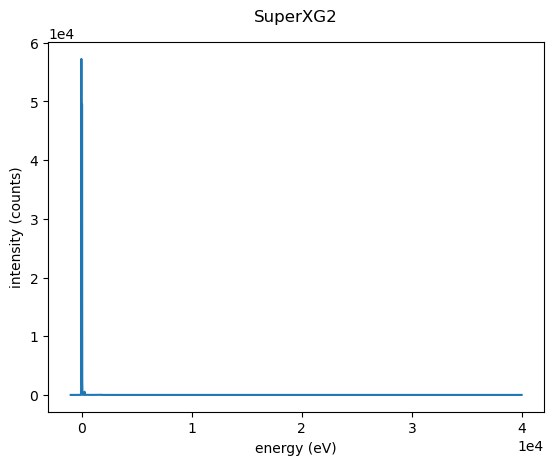
spectrum1 =tags[0]['data']
spectrum2 =tags[1]['data']
offset = float(tags[0]['spectrum_header']['CalibAbs'])
scale  = float(tags[0]['spectrum_header']['CalibLin'])
energy_scale1 = np.arange(len(spectrum1))*scale+offset
offset = float(tags[1]['spectrum_header']['CalibAbs'])
scale  = float(tags[1]['spectrum_header']['CalibLin'])
energy_scale2 = np.arange(len(spectrum2))*scale+offset
plt.figure()
plt.plot(energy_scale1,spectrum1, label = 'spectrum 1')
plt.plot(energy_scale2,spectrum2, label = 'spectrum 2')
plt.gca().set_xlabel('energy [keV]');
print(tags['overlay'].keys())
print(tags['overlay']['image1'])
#print(tags['3']['hardware_header'])
print(tags['detector'])
print(tags['esma'])
#print(tags['3']['spectrum_header'])
dict_keys(['image1', 'image2'])
{'Spectrum 1': {'posX': 483, 'posY': 504}, 'Spectrum 2': {'posX': 191, 'posY': 277}}
{'TRTKnownHeader': '\n                ', 'Technology': 'SDDpr', 'Serial': '11960', 'Type': 'XFlash 6|30', 'DetectorThickness': 0.045000000000000005, 'SiDeadLayerThickness': 2.9e-08, 'DetLayers': 'eJyzcUkt8UmsTC0qtrMB0wYKjiX5ubZKhsZKCiEZmcnZeanFxbZKpq66xkr6UDWGUDXmKEos9ICKjOCKjKCKTFEUmSGbYwxVYoZbiQlUiQWqErhV+gj3AwCpRT07', 'WindowType': 'slew AP3.3', 'window': {'Layer0': {'Z': '5', 'thickness': 1.3e-07}, 'Layer1': {'Z': '6', 'thickness': 1.45e-06}, 'Layer2': {'Z': '7', 'thickness': 4.5000000000000003e-07}, 'Layer3': {'Z': '8', 'thickness': 8.500000000000001e-07}, 'Layer4': {'Z': '13', 'thickness': 3.5000000000000004e-07}, 'Layer5': {'Z': '14', 'thickness': 0.0038000000000000004, 'relative_area': 0.23}}, 'CorrectionType': '3', 'ResponseFunctionCount': '21', 'SampleCount': '5', 'SampleOffset': '-3', 'PulsePairResTimeCount': '8', 'PileUpMinEnergy': '4.00000006E-1', 'PileUpWithBG': '1', 'TailFactor': '1', 'ShelfFactor': '1', 'ShiftFactor': '3.720000088E-1', 'ShiftFactor2': '-8.500000238E-1', 'ShiftData': '0.069977,0.005798,0.182983,0.007797,0.276978,0.005798,0.554932,0,1.099609,0,3.292969,0.006397,5.888672,0,0,0,0,0,', 'PPRTData': '0.95,2.891959,1.05,2.195911,1.55,1.700256,1.75,1.604574,3.75,1.155987,4.55,0.980248,5.95,1.003,8.05,1.004377,'}
{'PrimaryEnergy': 20.0, 'ElevationAngle': 35.0, 'AzimutAngle': 45.0, 'Magnification': 2274.1145, 'WorkingDistance': 8.9591}
plt.figure(figsize=(10,4))

ax1 = plt.subplot(1,2,1)
ax1.imshow(tags['image']['0']['data']['0'])
for key in tags['overlay']['image1']:
    d = tags['overlay']['image1'][key]
    ax1.scatter ([d['posX']], [d['posY']], marker="x", color='r')
    ax1.text(d['posX']+5, d['posY']-5, key, color='r')

ax2 = plt.subplot(1,2,2)
plt.plot(energy_scale1,spectrum1, label = 'spectrum 1')
plt.plot(energy_scale2,spectrum2, label = 'spectrum 2')
plt.gca().set_xlabel('energy [keV]')
plt.xlim(0,5)
plt.ylim(0)
plt.tight_layout()
plt.legend();
4.19.4. Find Maximas#
Of course we can find the maxima with the first derivative
from scipy.interpolate import InterpolatedUnivariateSpline

# Get a function that evaluates the linear spline at any x
f = InterpolatedUnivariateSpline(energy_scale1,spectrum1, k=1)

# Get a function that evaluates the derivative of the linear spline at any x
dfdx = f.derivative()

# Evaluate the derivative dydx at each x location...
dydx = dfdx(energy_scale1)
from scipy.ndimage import gaussian_filter


plt.figure()
plt.plot(energy_scale1,spectrum1, label = 'spectrum 1')

#plt.plot(energy_scale1, dydx)
plt.plot(energy_scale1,gaussian_filter(dydx, sigma=3)/10)
plt.gca().axhline(y=0,color='gray')
plt.gca().set_xlabel('energy [keV]');
4.19.5. Peak Finding#
We can also use the peak finding routine of the scipy.signal to find all the maxima.
import scipy as sp
import scipy.signal as sig

start = np.searchsorted(energy_scale1, 0.125)
## we use half the width of the resolution for smearing
width = int(np.ceil(125*1e-3/2 /(energy_scale1[1]-energy_scale1[0])/2)*2+1)
new_spectrum =  sp.signal.savgol_filter(spectrum1[start:], width, 2) ## we use half the width of the resolution for smearing
new_energy_scale = energy_scale1[start:]
major_peaks, _  = sp.signal.find_peaks(new_spectrum, prominence=1000)
minor_peaks, _  = sp.signal.find_peaks(new_spectrum, prominence=30)
peaks = major_peaks

spectrum1 = np.array(spectrum1)
plt.figure()
plt.plot(energy_scale1,spectrum1, label = 'spectrum 1')
#plt.plot(energy_scale1,gaussian_filter(spectrum1, sigma=1), label = 'filtered spectrum 1')
plt.plot(new_energy_scale,new_spectrum, label = 'filtered spectrum 1')
plt.scatter( new_energy_scale[minor_peaks], new_spectrum[minor_peaks], color = 'blue')
plt.scatter( new_energy_scale[major_peaks], new_spectrum[major_peaks], color = 'red')

plt.xlim(.126,5);
4.19.6. Peak identification#
Here we look up all the elemetns and see whether the position of major line (K-L3, K-L2’ or ‘L3-M5’) coincides with a peak position as found above.
Then we plot all the lines of such an element with the appropriate weight.
The positions and the weight are tabulated in the ffast.pkl file introduced in the Characteristic X-Ray peaks notebook
import pickle
pkl_file = open('data/ffast.pkl', 'rb')
ffast = pickle.load(pkl_file)
pkl_file.close()

plt.figure()
#plt.plot(energy_scale1,spectrum2, label = 'spectrum 1')
#plt.plot(energy_scale1,gaussian_filter(spectrum1, sigma=1), label = 'filtered spectrum 1')
plt.plot(new_energy_scale,new_spectrum, label = 'filtered spectrum 1')
plt.xlim(0.1,4)
plt.ylim(-800)
plt.gca().axhline(y=0,color='gray',  linewidth = 0.5);

out_tags = {}
out_tags['spectra'] = {}

out_tags['spectra'][0] = {}
out_tags['spectra'][0]['data'] = spectrum1
out_tags['spectra'][0]['energy_scale'] = energy_scale1
out_tags['spectra'][0]['energy_scale_start'] = start
out_tags['spectra'][0]['smooth_spectrum'] = new_spectrum
out_tags['spectra'][0]['smooth_energy_scale'] = new_energy_scale

out_tags['spectra'][0]['elements'] ={}


#print(ffast[6])
number_of_elements = 0
for peak in minor_peaks:
    for element in range(1,93):
        if 'K-L3' in ffast[element]['lines']:
            if abs(ffast[element]['lines']['K-L3']['position']- new_energy_scale[peak]*1e3) <10:
                out_tags['spectra'][0]['elements'][number_of_elements] = {}
                out_tags['spectra'][0]['elements'][number_of_elements]['element'] = ffast[element]['element']
                out_tags['spectra'][0]['elements'][number_of_elements]['found_lines'] = 'K-L3'
                out_tags['spectra'][0]['elements'][number_of_elements]['lines'] = ffast[element]['lines']
                out_tags['spectra'][0]['elements'][number_of_elements]['experimental_peak_index'] = peak
                out_tags['spectra'][0]['elements'][number_of_elements]['experimental_peak_energy'] = new_energy_scale[peak]*1e3
                number_of_elements += 1
                plt.plot([ffast[element]['lines']['K-L3']['position']/1000.,ffast[element]['lines']['K-L3']['position']/1000.], [0,new_spectrum[peak]], color = 'red')
                plt.text(new_energy_scale[peak],0, ffast[element]['element']+'\nK-L3', verticalalignment='top')
                for line in ffast[element]['lines']:
                    if 'K' in line:
                        if abs(ffast[element]['lines'][line]['position']-ffast[element]['lines']['K-L3']['position'])> 20:
                            if ffast[element]['lines'][line]['weight']>0.07:
                                #print(element, ffast[element]['lines'][line],new_spectrum[peak]*ffast[element]['lines'][line]['weight'])
                                plt.plot([ffast[element]['lines'][line]['position']/1000.,ffast[element]['lines'][line]['position']/1000.], [0,new_spectrum[peak]*ffast[element]['lines'][line]['weight']], color = 'red')
                                plt.text(ffast[element]['lines'][line]['position']/1000.,0, ffast[element]['element']+'\n'+line, verticalalignment='top')

        elif 'K-L2' in ffast[element]['lines']:
            if abs(ffast[element]['lines']['K-L2']['position']- new_energy_scale[peak]*1e3) <10:
                plt.plot([new_energy_scale[peak],new_energy_scale[peak]], [0,new_spectrum[peak]], color = 'orange')
                plt.text(new_energy_scale[peak],0, ffast[element]['element']+'\nK-L2', verticalalignment='top')
                out_tags['spectra'][0]['elements'][number_of_elements] = {}
                out_tags['spectra'][0]['elements'][number_of_elements]['element'] = ffast[element]['element']
                out_tags['spectra'][0]['elements'][number_of_elements]['found_lines'] = 'K-L2'
                out_tags['spectra'][0]['elements'][number_of_elements]['lines'] = ffast[element]['lines']
                out_tags['spectra'][0]['elements'][number_of_elements]['experimental_peak_index'] = peak
                out_tags['spectra'][0]['elements'][number_of_elements]['experimental_peak_energy'] = new_energy_scale[peak]*1e3

                number_of_elements += 1
        if 'L3-M5' in ffast[element]['lines']:
            if abs(ffast[element]['lines']['L3-M5']['position']- new_energy_scale[peak]*1e3) <10:
                pass
                print('found_element', element,ffast[element]['lines']['L3-M5']['position'], new_energy_scale[peak] )
                #plt.scatter( new_energy_scale[peak], new_spectrum[peak], color = 'blue')
                out_tags['spectra'][0]['elements'][number_of_elements] = {}
                out_tags['spectra'][0]['elements'][number_of_elements]['element'] = ffast[element]['element']
                out_tags['spectra'][0]['elements'][number_of_elements]['found_lines'] = 'L3-M5'
                out_tags['spectra'][0]['elements'][number_of_elements]['lines'] = ffast[element]['lines']
                out_tags['spectra'][0]['elements'][number_of_elements]['experimental_peak_index'] = peak
                out_tags['spectra'][0]['elements'][number_of_elements]['experimental_peak_energy'] = new_energy_scale[peak]*1e3

                number_of_elements += 1
for element in out_tags['spectra'][0]['elements']:
    print(out_tags['spectra'][0]['elements'][element]['element'],out_tags['spectra'][0]['elements'][element]['found_lines'])
found_element 51 3604.7 3.597909755
C K-L2
O K-L3
Mg K-L3
Al K-L3
P K-L3
S K-L3
K K-L3
Sb L3-M5
print(out_tags['spectra'][0]['elements'][0])#['K-L2']['weight'] = 0.5
#del out_tags['spectra'][0]['elements'][7]
for ele in out_tags['spectra'][0]['elements']:
    print(out_tags['spectra'][0]['elements'][ele]['element'])
{'element': 'C', 'found_lines': 'K-L2', 'lines': {'K-L2': {'weight': 0.5, 'position': 277.40000000000003}}, 'experimental_peak_index': 30, 'experimental_peak_energy': 277.577755}
C
O
Mg
Al
P
S
K
Sb
4.19.7. Plotting Gaussians in the Peaks#
Please note the different width (FWHM). Here I guessed the peak width for two peaks.
def gaussian(enrgy_scale, mu, FWHM):
    sig = FWHM/2/np.sqrt(2*np.log(2))
    return np.exp(-np.power(enrgy_scale - mu, 2.) / (2 * np.power(sig, 2.)))

C_peak = gaussian(new_energy_scale, .275, .068)
P_peak = gaussian(new_energy_scale, 2.019, .095)
plt.figure()

plt.plot(new_energy_scale,new_spectrum, label = 'spectrum')
plt.plot(new_energy_scale,C_peak*8233, label = 'C peak')
plt.plot(new_energy_scale,P_peak*8000, label = 'P peaks', color = 'red')
plt.xlim(.1,3)
plt.legend()
<matplotlib.legend.Legend at 0x1e4095b53d0>
4.19.8. Origin of Line Width#
Electron hole pairs are created with a standard deviation corresponding to the quantum mechanical shot-noise (Poisson statistic).
The distribution is then a Gaussian with the width of the standard deviation
For the Mn K-L2,3 peak< this width would be 40 electron hole pairs. The full width at half maximum (FWHM) of the Mn K-L2,3 edge would then be (FWHM of Gaussian is 2.35 * 𝜎) about 106 eV a major component of the observed 125 eV in good EDS systems.
4.19.9. Line Width Estimate#
Fiori and Newbury 1978
From a reference peak at
Gernerally we use the Mn K-L2,3 peak
E_ref = 5895.0
FWHM_ref = 136 #eV
E= 275
def getFWHM(E):
    return np.sqrt(2.5*(E-E_ref)+FWHM_ref**2)

print(getFWHM(E))
66.6783323126786
Using that we get for all peaks in the low energy region:
def getPeak(E, energy_scale):
    E_ref = 5895.0
    FWHM_ref = 136 #eV
    FWHM  = np.sqrt(2.5*(E*1e3-E_ref)+FWHM_ref**2)*1e-3
    return gaussian(energy_scale, E, FWHM)

E= .275
C_peak = getPeak(E,new_energy_scale)
E = 2.019
P_peak = getPeak(E,new_energy_scale)
E = 1.258
Al_peak = getPeak(E,new_energy_scale)
E = 0.528
O_peak = getPeak(E,new_energy_scale)
plt.figure()

plt.plot(new_energy_scale,new_spectrum, label = 'filtered spectrum 1')
plt.plot(new_energy_scale,C_peak*8233, label = 'filtered spectrum 1')
plt.plot(new_energy_scale,P_peak*8000, label = 'filtered spectrum 1')
plt.plot(new_energy_scale,Al_peak*4600, label = 'filtered spectrum 1')

plt.plot(new_energy_scale,O_peak*4600, label = 'filtered spectrum 1')
plt.xlim(.1,3)
C:\Users\gduscher\AppData\Local\Temp\ipykernel_51724\2131547806.py:15: RuntimeWarning: More than 20 figures have been opened. Figures created through the pyplot interface (`matplotlib.pyplot.figure`) are retained until explicitly closed and may consume too much memory. (To control this warning, see the rcParam `figure.max_open_warning`). Consider using `matplotlib.pyplot.close()`.
  plt.figure()
(0.1, 3.0)
4.19.10. Detector Efficiency#
from scipy.interpolate import interp1d
import scipy.constants as const


## layer thicknesses of commen materials in EDS detectors in m
nickelLayer = 0.* 1e-9 # in m
alLayer = 30 *1e-9    # in m
C_window = 2 *1e-6    # in m
goldLayer = 0.* 1e-9   # in m
deadLayer = 100 *1e-9  # in m
detector_thickness = 45 * 1e-3  # in m

area = 30 * 1e-6 #in m2
oo4pi = 1.0 / (4.0 * np.pi)

#We make a linear energy scale
energy_scale = np.linspace(.1,60,2000)

## interpolate mass absorption coefficient to our energy scale
lin = interp1d(ffast[14]['E']/1000.,ffast[14]['photoabsorption'],kind='linear')
mu_Si = lin(energy_scale) * ffast[14]['nominal_density']*100. #1/cm -> 1/m

## interpolate mass absorption coefficient to our energy scale
lin = interp1d(ffast[13]['E']/1000.,ffast[13]['photoabsorption'],kind='linear')
mu_Al = lin(energy_scale) * ffast[13]['nominal_density'] *100. #1/cm -> 1/m

lin = interp1d(ffast[6]['E']/1000.,ffast[6]['photoabsorption'],kind='linear')
mu_C = lin(energy_scale) * ffast[6]['nominal_density'] *100. #1/cm -> 1/m

detector_Efficiency1 = np.exp(-mu_C * C_window) * np.exp(-mu_Al * alLayer)* np.exp(-mu_Si * deadLayer)
detector_Efficiency2 = (1.0 - np.exp(-mu_Si * detector_thickness))# * oo4pi;
detector_Efficiency =detector_Efficiency1 * detector_Efficiency2#* oo4pi;

plt.figure()
plt.plot(energy_scale, detector_Efficiency*100, label = 'total absorption')
plt.plot(energy_scale, detector_Efficiency1*100, label = 'detector absorption')
plt.plot(energy_scale, detector_Efficiency2*100, label= 'detector efficiency')
plt.gca().set_xlabel('energy [keV]');
plt.gca().set_ylabel('efficiency [%]')
plt.legend();
energy_scale = new_energy_scale
4.19.11. Detector Parameters from file#
print(tags['detector']['window'])
print(tags['detector'].keys())
print(f"{float(tags['detector']['SiDeadLayerThickness'])*1e-6:.3g}")
print(f"{float(tags['detector']['DetectorThickness'])/10:.3f}")
for key in tags['detector']['window']:
    print(f"{tags['detector']['window'][key]['Z']}, {tags['detector']['window'][key]['thickness']*1e-6:.2g}")
{'Layer0': {'Z': '5', 'thickness': 1.3e-07}, 'Layer1': {'Z': '6', 'thickness': 1.45e-06}, 'Layer2': {'Z': '7', 'thickness': 4.5000000000000003e-07}, 'Layer3': {'Z': '8', 'thickness': 8.500000000000001e-07}, 'Layer4': {'Z': '13', 'thickness': 3.5000000000000004e-07}, 'Layer5': {'Z': '14', 'thickness': 0.0038000000000000004, 'relative_area': 0.23}}
dict_keys(['TRTKnownHeader', 'Technology', 'Serial', 'Type', 'DetectorThickness', 'SiDeadLayerThickness', 'DetLayers', 'WindowType', 'window', 'CorrectionType', 'ResponseFunctionCount', 'SampleCount', 'SampleOffset', 'PulsePairResTimeCount', 'PileUpMinEnergy', 'PileUpWithBG', 'TailFactor', 'ShelfFactor', 'ShiftFactor', 'ShiftFactor2', 'ShiftData', 'PPRTData'])
2.9e-14
0.005
5, 1.3e-13
6, 1.5e-12
7, 4.5e-13
8, 8.5e-13
13, 3.5e-13
14, 3.8e-09
4.19.12. Comparison to generic efficiency#
from scipy.interpolate import interp1d
import scipy.constants as const

def detector_efficiency(tags, energy_scale):
    detector_Efficiency1 = np.ones(len(energy_scale))
    for key in tags['detector']['window']:
        Z = int(tags['detector']['window'][key]['Z'])
        if Z < 14:
            t = tags['detector']['window'][key]['thickness']

            ## interpolate mass absorption coefficient to our energy scale
            lin = interp1d(ffast[Z]['E']/1000.,ffast[Z]['photoabsorption'],kind='linear')
            mu = lin(energy_scale) * ffast[Z]['nominal_density']*100. #1/cm -> 1/m
            detector_Efficiency1 = detector_Efficiency1 * np.exp(-mu * t)
            print(Z,t)

    t = float(tags['detector']['SiDeadLayerThickness'])*1e-6
    print(t)
    t = .30*1e-7
    print(t)
    lin = interp1d(ffast[14]['E']/1000.,ffast[14]['photoabsorption'],kind='linear')
    mu = lin(energy_scale) * ffast[14]['nominal_density']*100. #1/cm -> 1/m
    detector_Efficiency1 = detector_Efficiency1 * np.exp(-mu * t)
    detector_thickness = float(tags['detector']['DetectorThickness'])*1e-1
    ## interpolate mass absorption coefficient to our energy scale
    mu_Si = lin(energy_scale) * ffast[14]['nominal_density']*100. #1/cm -> 1/m
    print(detector_thickness)

    detector_Efficiency2 = (1.0 - np.exp(-mu * detector_thickness))# * oo4pi;


    return detector_Efficiency1*detector_Efficiency2
de = detector_efficiency(tags, energy_scale)
## layer thicknesses of commen materials in EDS detectors in m
nickelLayer = 0.* 1e-9 # in m
alLayer = 30 *1e-9    # in m
C_window = 2 *1e-6    # in m
goldLayer = 0.* 1e-9   # in m
deadLayer = 100 *1e-9  # in m
detector_thickness = 45 * 1e-3  # in m
print(detector_thickness)
area = 30 * 1e-6 #in m2
oo4pi = 1.0 / (4.0 * np.pi)

#We make a linear energy scale
energy_scale = new_energy_scale


## interpolate mass absorption coefficient to our energy scale
lin = interp1d(ffast[14]['E']/1000.,ffast[14]['photoabsorption'],kind='linear')
mu_Si = lin(energy_scale) * ffast[14]['nominal_density']*100. #1/cm -> 1/m

## interpolate mass absorption coefficient to our energy scale
lin = interp1d(ffast[13]['E']/1000.,ffast[13]['photoabsorption'],kind='linear')
mu_Al = lin(energy_scale) * ffast[13]['nominal_density'] *100. #1/cm -> 1/m

lin = interp1d(ffast[6]['E']/1000.,ffast[6]['photoabsorption'],kind='linear')
mu_C = lin(energy_scale) * ffast[6]['nominal_density'] *100. #1/cm -> 1/m

detector_Efficiency1 = np.exp(-mu_C * C_window) * np.exp(-mu_Al * alLayer)#* np.exp(-mu_Si * deadLayer)
detector_Efficiency2 = (1.0 - np.exp(-mu_Si * detector_thickness))# * oo4pi;
detector_Efficiency =detector_Efficiency1 * detector_Efficiency2#* oo4pi;

plt.figure()
plt.plot(energy_scale*1000, detector_Efficiency , label = 'generic')
plt.plot(energy_scale*1000, de, label = 'UTK detector')
#plt.plot(energy_scale*1000, de* np.exp(-mu_Si * deadLayer) )
#plt.plot(energy_scale*1000, de* np.exp(-mu_Si * deadLayer) * detector_Efficiency2 )
plt.legend();
plt.xlim(0,9000);
5 1.3e-07
6 1.45e-06
7 4.5000000000000003e-07
8 8.500000000000001e-07
13 3.5000000000000004e-07
2.9e-14
3e-08
0.0045000000000000005
0.045
4.19.13. Plotting background and lines#
Peaks = []
elements_peaks = []
intensities = []
for element in out_tags['spectra'][0]['elements']:
    el_dict = out_tags['spectra'][0]['elements'][element]

    position = el_dict['lines'][el_dict['found_lines']]['position']
    weight = 0
    for line in el_dict['lines']:
        if abs(position - el_dict['lines'][line]['position'])<20:
            weight += el_dict['lines'][line]['weight']
    index = np.searchsorted(new_energy_scale,el_dict['lines'][el_dict['found_lines']]['position']/1000.)
    intensity = new_spectrum[index]/weight
    added_peaks = np.zeros(len(new_energy_scale))
    for line in el_dict['lines']:
        if line[0] == el_dict['found_lines'][0]:
            if el_dict['lines'][line]['weight']> 0.01:
                p = getPeak(el_dict['lines'][line]['position']/1000.,new_energy_scale)*el_dict['lines'][line]['weight']
                Peaks.append(p)
                added_peaks = added_peaks + p
    elements_peaks.append(added_peaks)
    intensities.append(intensity)

plt.figure()
plt.plot(new_energy_scale,new_spectrum, label = 'filtered spectrum 1')
#plt.plot(new_energy_scale,new_spectrum, label = 'filtered spectrum 1',color='red')
for i in range(len(elements_peaks)):
    plt.plot(new_energy_scale,elements_peaks[i]*intensities[i], label = f'Peak{i}')
    pass
peaks = np.array(Peaks)
plt.plot(new_energy_scale,peaks.sum(axis=0), label = f'Peaks', color = 'blue')
print(peaks.shape)
#plt.xlim(0,5)
offset = float(tags[0]['spectrum_header']['CalibAbs'])
scale  = float(tags[0]['spectrum_header']['CalibLin'])
energy_scale1 = np.arange(len(spectrum1))*scale+offset
p = [1, 37, .3, offset, scale]
E_0= 20
E = new_energy_scale
N = detector_Efficiency * (p[0] + p[1]*(E_0-E)/E + p[2]*(E_0-E)**2/E)
N = de * (p[0] + p[1]*(E_0-E)/E + p[2]*(E_0-E)**2/E)

pp = p[0:5].copy()
for i in range(len(elements_peaks)):
    pp.append(intensities[i])

plt.plot(new_energy_scale,N, color= 'orange')

plt.xlim(0,4)

detector_Efficiency = de
(29, 3922)
detector_Efficiency.shape
(2000,)
4.19.14. As a function#
def model(p,energy_scale):
    E = energy_scale

    spectrum = detector_Efficiency * (p[0] + p[1]*(E_0-E)/E + p[2]*(E_0-E)**2/E)

    for i in range(5,len(p)):
        spectrum = spectrum+elements_peaks[i-5]*abs(p[i])
    return spectrum
spectrum3 = model(pp[:-1],new_energy_scale)

plt.figure()

plt.plot(new_energy_scale,new_spectrum, label = 'filtered spectrum 1',color='red')
plt.plot(new_energy_scale, spectrum3)
plt.xlim(0,4)
(0.0, 4.0)
4.19.15. Fitting above function to spectrum#
from scipy.optimize import leastsq

## background fitting
def specfit(p, y, x):
    err = y - model(p,x)
    return err

p, lsq = leastsq(specfit, pp[:-1], args=(new_spectrum, new_energy_scale), maxfev=2000)
print( f'element\t end   \t   start ')
for i, element in enumerate(out_tags['spectra'][0]['elements']):
    if i<len(p)-5:
        el_dict = out_tags['spectra'][0]['elements'][element]
        print(f"{el_dict['element']:2s}: \t  {abs(p[i+5]):6.2f} \t  {pp[i+5]:.2f}")
#print(p,pp)
element	 end   	   start
C : 	  16487.64 	  16444.49
O : 	  3267.00 	  3274.63
Mg: 	  2831.85 	  3127.80
Al: 	   84.40 	  334.63
P : 	  5267.50 	  5499.66
S : 	   82.35 	  234.96
K : 	  2526.57 	  2693.25
spectrum3 = model(p,new_energy_scale)

plt.figure()

plt.plot(new_energy_scale,new_spectrum, label = 'filtered spectrum 1',color='red')
plt.plot(new_energy_scale, spectrum3)
plt.plot(new_energy_scale, new_spectrum-spectrum3)
plt.gca().axhline(y=0,color='gray');

plt.xlim(0,4);
4.19.16. Energy Scale#
What happened?
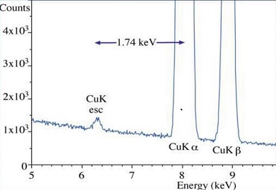
4.19.17. Detector Artifacts#
4.19.17.1. Si Escape peak#
The 1s state of a Si atom in the detector crystal is excited but then instead of being further detected by absoption a A!!uger electron leaves the crystal. The electron hole pairs of this event are missing and a lower energy is recorded.
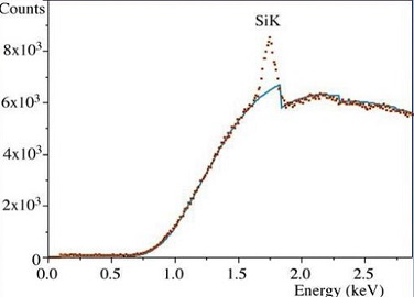
4.19.17.2. Detector Silicon Peak#
Internal fluorescence peak
4.19.17.3. Sum Peak#
Two photons are detected at the same time. This signal is suppressed by most acquistion systems, but a few are still slipping through. A peak apears at the energy of the sum of two strong peaks.
4.19.18. Composition#
Following
to calculate the mass concentration
where:
What do we know at this point?
def BrowningEmpiricalCrossSection(elm , energy):
""" * Computes the elastic scattering cross section for electrons of energy between
* 0.1 and 30 keV for the specified element target. The algorithm comes from<br>
* Browning R, Li TZ, Chui B, Ye J, Pease FW, Czyzewski Z & Joy D; J Appl
* Phys 76 (4) 15-Aug-1994 2016-2022
* The implementation is designed to be similar to the implementation found in
* MONSEL.
* Copyright: Pursuant to title 17 Section 105 of the United States Code this
* software is not subject to copyright protection and is in the public domain
* Company: National Institute of Standards and Technology
* @author Nicholas W. M. Ritchie
* @version 1.0
*/
Modified by Gerd Duscher, UTK
"""
#/**
#* totalCrossSection - Computes the total cross section for an electron of
#* the specified energy.
#*
# @param energy double - In keV
# @return double - in square meters
#*/
e = energy #in keV
re = np.sqrt(e);
return (3.0e-22 * elm**1.7) / (e + (0.005 * elm**1.7 * re) + ((0.0007 * elm**2) / re));
print(BrowningEmpiricalCrossSection(6,277)*1e18, r'nm^2')
2.2633981858464282e-05 nm^2