Chapter 2: Diffraction
2.11. Kikuchi Lines#
![]()
part of
MSE672: Introduction to Transmission Electron Microscopy
Spring 2025
by Gerd Duscher
Microscopy Facilities
Institute of Advanced Materials & Manufacturing
Materials Science & Engineering
The University of Tennessee, Knoxville
Background and methods to analysis and quantification of data acquired with transmission electron microscopes
2.11.1. Load relevant python packages#
2.11.1.1. Check Installed Packages#
import sys
import importlib.metadata
def test_package(package_name):
    """Test if package exists and returns version or -1"""
    try:
        version = importlib.metadata.version(package_name)
    except importlib.metadata.PackageNotFoundError:
        version = '-1'
    return version

if test_package('pyTEMlib') < '0.2024.1.0':
    print('installing pyTEMlib')
    !{sys.executable} -m pip install git+https://github.com/pycroscopy/pyTEMlib.git@main -q --upgrade

if 'google.colab' in sys.modules:
    !{sys.executable} -m pip install numpy==1.24.4
print('done')
2.11.1.2. Load the plotting and figure packages#
Import the python packages that we will use:
Beside the basic numerical (numpy) and plotting (pylab of matplotlib) libraries,
itertools (iterations of variables here to generate all possible Miller indices)
scipy.constants (all physical constants from scientific library scipy) some libraries from the book
kinematic scattering library.
diffraction_plot (which could be accessed through the scatteering library)
%matplotlib  widget
import matplotlib.pyplot as plt
import numpy as np
import sys
if 'google.colab' in sys.modules:
    from google.colab import output
    output.enable_custom_widget_manager()

# 3D plotting package used
from mpl_toolkits.mplot3d import Axes3D # 3D plotting

# additional package
import itertools
import scipy.constants as const

# Import libraries from the pyTEMlib
import pyTEMlib
import pyTEMlib.kinematic_scattering as ks         # Kinematic sCattering Library
                             # Atomic form factors from Kirklands book
from pyTEMlib import diffraction_plot as diff_plot

__notebook_version__ = '2025.02.11'

print('pyTEM version: ', pyTEMlib.__version__)
print('notebook version: ', __notebook_version__)
You don't have igor2 installed.     If you wish to open igor files, you will need to install it     (pip install igor2) before attempting.
You don't have gwyfile installed.     If you wish to open .gwy files, you will need to      install it (pip install gwyfile) before attempting.
Symmetry functions of spglib enabled
Using kinematic_scattering library version {_version_ }  by G.Duscher
pyTEM version:  0.2024.09.0
notebook version:  2025.02.11
2.11.2. Kikuchi Pattern#
An electron can be scattered elastically into the Bragg angle, or it can be scattered inelastically
The inelastically scattered electrons are emitted in all directions.
These inelastically scattered electrons are then diffracted at the crystal planes according to Bragg’s law.
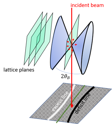
This results in a cone, where the Bragg diffraction is allowed; this cone is called Kossel cone. Because the electrons are predominantly scattered in the direction of the incident beam, this Bragg diffraction will take some intensity out of the original beam (dark line: deficit line in the figure )and transfer it to a different angle (bright band: excess line in the figure. Inside this bands is some intensity which depends on the dynamic scattering.
The most important feature of the Kikuchi band is that the Kossel cones are fixed to the crystal and allow easy navigation in reciprocal space, because nothing changes with the angle (the excitation error and thickness changes for SAD patterns). A common example if you want to tilt out of a zone axis, but you also want to keep an interface edge on; you just follow the Kikuchi band of the interface plane.
Note:
the Kikuchi bands are bent, they just appear straight, because the Ewald sphere is so large.
Note:
According to the explanation above, no Kikuchi lines should be visible if we are in a low order zone axis. This is not true because of the channeling effect and dynamic scattering, but these effects do not change anything about the location, where we expect the Kikuchi lines.
2.11.3. Constructing Kikuchi Maps#
2.11.3.1. Define crystal#
### Please choose another crystal like: Silicon, Aluminium, GaAs , ZnO
atoms = ks.structure_by_name('silicon')
atoms
Lattice(symbols='Si8', pbc=True, cell=[5.43088, 5.43088, 5.43088])
2.11.3.2. Plot the unit cell#
Just to be sure the crystal structure is right
from ase.visualize.plot import plot_atoms

plot_atoms(atoms, radii=0.3, rotation=('0x,4y,0z'))
<Axes: >
2.11.3.3. Parameters for Diffraction Calculation#
Please note that we are using a rather small number of reflections: the maximum number of Miller indices
maximum hkl is 1
tags = {}
atoms.info['experimental'] = {'acceleration_voltage_V': 20.0 *1000.0, #V
                              'convergence_angle_mrad': 0,
                              'zone_hkl': np.array([0,1,1]),  # incident neares zone axis: defines Laue Zones!!!!
                              'Sg_max': 0.05, # 1/Ang  maximum allowed excitation error ; This parameter is related to the thickness
                              'hkl_max': 1 }  # Highest evaluated Miller indices
2.11.3.4. Calculation#
ks.kinematic_scattering(atoms, False)
The results are in the info attribute as a dictionary in atoms.info[‘diffraction’]
2.11.3.5. Plot Selected Area Electron Diffraction Pattern#
# ########################
# Plot ZOLZ SAED Pattern #
# ########################

# Get information as dictionary
diffraction = atoms.info['diffraction']
#We plot only the allowed diffraction spots
points = diffraction['allowed']['g']
# we sort them by order of Laue zone
ZOLZ = diffraction['allowed']['ZOLZ']

# Plot
fig = plt.figure()
ax = fig.add_subplot(111)
# We plot the x,y axis only; the z -direction is set to zero - this is our projection
ax.scatter(points[ZOLZ,0], points[ZOLZ,1], c='red', s=40)

# zero spot plotting
ax.scatter(0,0, c='red', s=100)
ax.scatter(0,0, c='white', s=40)

ax.axis('equal')
FOV = .3
plt.ylim(-FOV,FOV); plt.xlim(-FOV,FOV);
2.11.4. Kikuchi Line Construction#
The Kikuchi lines are the Bisections of lines from the center spot to the Bragg spots.
The line equation for a bisection of a line between two points
If
In our case point
If
pointsZ = points[ZOLZ]

g = pointsZ[1,0:2]

x_A, y_A = g


slope = -x_A/y_A
y_0 = (x_A**2+ y_A**2)/(2*y_A)

# Starting point of Kikuchi Line
x1 = -FOV
y1 = y_0+slope*x1
# End point of Kikuchi Line
x2= FOV
y2 = y_0+slope*x2


print(([x1,x2],[y1,y2]))
# Plot
fig = plt.figure()
ax = fig.add_subplot(111)
# We plot the x,y axis only; the z -direction is set to zero - this is our projection
ax.scatter(points[ZOLZ,0], points[ZOLZ,1], c='red', s=20 , alpha = .3)
ax.scatter(g[0], g[1], c='red', s=40)
# Draw kikuchi
ax.plot([x1,x2],[y1,y2],c='r')
ax.text(g[0]/2+0.04,g[1]/2+0.05, 'Kikuchi',color ='r', rotation=37)
ax.plot([0,g[0]],[0,g[1]],c='black')

# zero spot plotting
ax.scatter(0,0, c='red', s=100)
ax.scatter(0,0, c='white', s=40)

ax.axis('equal')
FOV = .3
plt.ylim(-FOV,FOV); plt.xlim(-FOV,FOV); plt.show()
plt.ylabel('angle (1/$\AA$)' )
([-0.3, 0.3], [-0.016830320493786938, 0.4074337482181415])
Text(30.972222222222214, 0.5, 'angle (1/$\\AA$)')
Assume we have an SAD pattern, from experiment or simulation. Draw a line from the center to each ZOLZ diffraction spot and draw a line perpendicular to the first line at half the distance. We name the line with the same Miller indices as the spot. The distance between two pair of lines is then again
If we know in which direction the next low order zone axis is and how far we have to tilt to get to it, we can draw that pole too.
pointsZ = points[ZOLZ]

g = pointsZ[0,0:2]

x_A, y_A = g
print(x_A, y_A)
slope = -x_A/y_A
y_0 = (x_A**2+ y_A**2)/(2*y_A)

x1 = -FOV
y1 = y_0+slope*x1

x2= FOV
y2 = y_0+slope*x2


print(([x1,x2],[y1,y2]))
# Plot
fig = plt.figure()
ax = fig.add_subplot(111)
# We plot the x,y axis only; the z -direction is set to zero - this is our projection
ax.scatter(points[ZOLZ,0], points[ZOLZ,1], c='red', s=20 , alpha = .3)
ax.scatter(g[0], g[1], c='red', s=40)
ax.plot([x1,x2],[y1,y2],c='r')
ax.text(x1/2,g[1]/2-.5, 'Kikuchi',color ='r', rotation=52)
ax.plot([0,g[0]],[0,g[1]],c='black')

# Make right angle symbol
ax.scatter(g[0]/2, g[1]/2)
#ax.plot([g[0]/2*.09, g[0]/2*.9+.01], [g[1]/2*.9,g[1]/2*.9+.01],c='black')
#ax.plot([g[0]/2*.9, g[0]/2*.9+.01],[g[1]/2*1.1,g[1]/2*1.1-.01],c='black')

# zero spot plotting
ax.scatter(0,0, c='red', s=100)
ax.scatter(0,0, c='white', s=40)

ax.axis('equal')
FOV = .4
plt.ylim(-FOV,FOV); plt.xlim(-FOV,FOV); plt.show()
-0.18413222166573373 -0.2604022851495697
([-0.3, 0.3], [0.016830320493786938, -0.4074337482181415])
2.11.4.1. Plotting of Kikuchi Pattern#
pointsZ = points[ZOLZ]

g = pointsZ[:,0:2]

FOV = .4
slope = -g[:,0]/g[:,1]
y_0 = (g[:,0]**2+ g[:,1]**2)/(2*g[:,1])

x1 = -FOV
y1 = y_0+slope*x1

x2= FOV
y2 = y_0+slope*x2


# Plot
fig = plt.figure()
ax = fig.add_subplot(111)
# We plot the x,y axis only; the z -direction is set to zero - this is our projection
ax.scatter(points[ZOLZ,0], points[ZOLZ,1], c='red', s=20 )
ax.plot([x1,x2],[y1,y2],c='r', alpha = 0.5)


# zero spot plotting
ax.scatter(0,0, c='red', s=100)
ax.scatter(0,0, c='white', s=40)

ax.set_aspect('equal')
FOV = .6
plt.ylim(-FOV,FOV); plt.xlim(-FOV,FOV); plt.show()
2.11.5. Plotting of Whole Kikuchi Pattern#
with a few more Bragg peaks, so please increase hkl_max and see what happens!
# ------- Input -----------
hkl_max = 3
# -------------------------

tags = atoms.info['experimental']
tags['hkl_max'] = hkl_max
tags['crystal_name'] = 'silicon'
ks.kinematic_scattering(atoms, False)
tagsD = atoms.info['diffraction']

#We plot only the allowed diffraction spots
points = tagsD['allowed']['g']
# we sort them by order of Laue zone
ZOLZ = tagsD['allowed']['ZOLZ']

pointsZ = points[ZOLZ]
g = pointsZ[:,0:2]

FOV = .6

g[g[:,1] ==0. , 1] = 1e-12  # to avoid division by zero
slope = -g[:,0]/g[:,1]
y_0 = (g[:,0]**2+ g[:,1]**2)/(2*g[:,1])

x1 = -FOV
y1 = y_0+slope*x1
x2= FOV
y2 = y_0+slope*x2

# Plot
fig = plt.figure()
plt.title(f" {tags['crystal_name']} in {tags['zone_hkl']}")
ax = fig.add_subplot(111)
# We plot the x,y axis only; the z -direction is set to zero - this is our projection
ax.scatter(points[ZOLZ,0], points[ZOLZ,1], c='red', s=20 )
ax.plot([x1,x2],[y1,y2],c='r', alpha = 0.5)


# zero spot plotting
ax.scatter(0,0, c='red', s=100)
ax.scatter(0,0, c='white', s=40)

ax.set_aspect('equal')
FOV = .6
plt.ylim(-FOV,FOV); plt.xlim(-FOV,FOV); plt.show()
2.11.6. Plotting of Whole Kikuchi Pattern with kineamtic_scattering Library#
# -------- input ---------------
crystal_name = 'SrTiO3'
zone_axis = [0, 0, 1]
# ----------------------------
atoms = ks.structure_by_name(crystal_name)
atoms.info['experimental'] = {'crystal_name': crystal_name,
                              'acceleration_voltage_V': 200.0 *1000.0, #V
                              'convergence_angle_mrad': 0,
                              'Sg_max': .03,   # 1/Ang  maximum allowed excitation error ; This parameter is related to the thickness
                              'hkl_max': 9,   # Highest evaluated Miller indices
                              'zone_hkl': np.array(zone_axis),
                              'mistilt alpha degree': .0,  # -45#-35-0.28-1+2.42
                              'mistilt beta degree': 0.,
                              'plot_FOV': 2}

ks.kinematic_scattering(atoms)

atoms.info['output'].update(diff_plot.plotSAED_parameter())

atoms.info['output'].update({'plot Kikuchi': True,
                             'color Kikuchi': 'navy',
                             'background': 'gray',
                             'label size': 12,
                             'plot shift x': 0,
                             'plot shift y': 0,
                             'image gamma': 2,
                             'label color': 'skyblue',
                             'color zero': 'white',
                             'plot_labels': False})

############
## OUTPUT
############

diff_plot.plot_diffraction_pattern(atoms)
#plt.gca().set_xlim(-2,2)
#plt.gca().set_ylim(-2,2)
2.11.7. Mistilt in Kikuchi Pattern#
Becasue Kikuchi pattern are directly fixed to the crystal any mistiolt can immediately be detected
# -------Input ------ #
crystal_name = 'SrTiO3'
zone_axis = [0, 0, 1]
mistilt_alpha = 5  # in degree
mistilt_beta = -.0
# ------------------- #


# Crystal unit cell defintion

atoms2 = ks.structure_by_name(crystal_name)

atoms2.info['experimental'] = {'crystal_name': crystal_name,
                              'acceleration_voltage_V': 200.0 *1000.0, #V
                              'convergence_angle_mrad': 0.,
                              'Sg_max': .03,   # 1/Ang  maximum allowed excitation error ; This parameter is related to the thickness
                              'thickness': 20,  # in Ang
                              'hkl_max': 11,   # Highest evaluated Miller indices
                              'zone_hkl': np.array(zone_axis),
                              'mistilt_alpha degree': mistilt_alpha,
                              'mistilt_beta degree': mistilt_beta,
                              'plot_FOV': 2}

ks.kinematic_scattering(atoms2)

atoms2.info['output']=diff_plot.plotSAED_parameter()

atoms2.info['output'].update({'plot Kikuchi': False,
                             'color Kikuchi': 'navy',
                             'background': 'gray',
                             'label size': 12,
                             'plot shift x': 0,
                             'plot shift y': 0,
                             'image gamma': 2,
                             'label color': 'skyblue',
                             'color zero': 'white',
                             'plot_labels': False})


############
## OUTPUT
############

diff_plot.plot_diffraction_pattern(atoms2, grey=False)
#plt.gca().set_xlim(-2, 2)
#plt.gca().set_ylim(-2, 2)
2.11.8. Kikuchi Maps#
Extremly helpfull for tilting a sample to a different zone axis are maps of Kikuchi pattern as the one below.
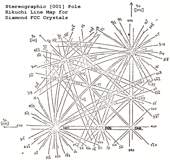
If you are in a specific zone axis, which we identify by its symmetry (like the SAED
2.11.9. Kikuchi Lines and Excitation Error#
Since the Kikuchi lines are rigidly attached to the crystal, we can use them to measure the excitation error. The diffraction geometry is shown in the figure above. If
# --- Input -----
s_g= -.05 # in 1/Ang
# ---------------

plt.figure()
from pyTEMlib import animation
animation.deficient_kikuchi_line(s_g= s_g)
Principle of excitation error determination. You can use this to obtain exact Bragg (s_g=0) conditions in your diffraction pattern.
2.11.10. Conclusion#
The Kikuchi lines are directly related to the Bragg reflections and therefore show the same symmetry as the diffraction pattern.
2.11.12. Appendix#
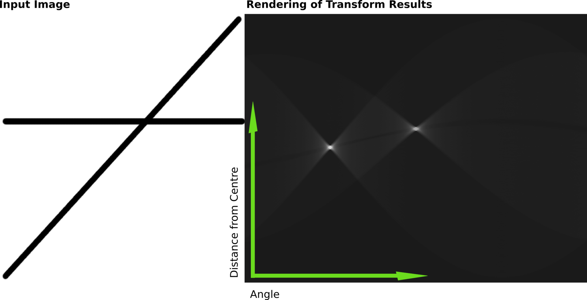
2.11.12.1. An Excursion to Hough space#
The line can be defined by
its end points
intersection with y and slope or
closest distance to origin and angle with x-axis.
The latter is called Hough Space and when we look at the Kikuchi construction we see that this is easily accomplished in that case:
The closest distance to origin is half the distance to the Bragg reflection.
The angle between the x-axis and the angle to the Bragg reflection plus 90
That means that polar coordinates and Hough space are closely related
points_polar = np.array([np.linalg.norm(points[:,:2], axis=1), np.arctan2(points[:,1],points[:,0])], dtype=float).T
points_polar
array([[ 0.31892636, -2.18627604],
       [ 0.31892636,  2.18627604],
       [ 0.31892636, -0.95531662],
       [ 0.31892636,  0.95531662]])
def hough2cartesian(points_polar, maxlength = .4):
    """ converts polar coordinates to lines and cartesian points """
    dist = points_polar[:, 0]
    angle = points_polar[:, 1]

    (x0, y0) = dist/2 * np.array([np.cos(angle), np.sin(angle)])

    h_xp = x0 + maxlength * np.cos(angle- np.pi/2)
    h_yp = y0 + maxlength * np.sin( angle-np.pi/2)
    h_xm = x0 - maxlength * np.cos( angle-np.pi/2)
    h_ym = y0 - maxlength * np.sin( angle-np.pi/2)

    return h_xp, h_yp, h_xm, h_ym, x0*2, y0*2

def cartesian2hough(points, maxlength = .4):
    """ converts cartesian coordinates to lines and polar points """

    dist = np.linalg.norm(points[:,:2], axis=1)
    angle = np.arctan2(points[:,1],points[:,0])

    h_xp = points[:,0]/2 + maxlength * np.cos(angle-np.pi/2)
    h_yp = points[:,1]/2 + maxlength * np.sin(angle-np.pi/2)
    h_xm = points[:,0]/2 - maxlength * np.cos(angle-np.pi/2)
    h_ym = points[:,1]/2 - maxlength * np.sin(angle-np.pi/2)

    return h_xp, h_yp, h_xm, h_ym, dist, angle

points_polar = np.array([np.linalg.norm(points[:,:2], axis=1), np.arctan2(points[:,1],points[:,0])], dtype=float).T

hxp,hyp,hxm,hym, x0, y0 = hough2cartesian(points_polar)

plt.figure()
plt.scatter(x0, y0, c='red', s=20 , alpha = .3),
plt.scatter(0, 0, c='red', s=20 , alpha = .8),
for i in range(len(hxm)):
    plt.plot([hxm[i], hxp[i]], [hym[i], hyp[i]])
plt.gca().set_aspect('equal')

Polar coordinates allow us to rotate the diffraction pattern quite easily, just add a fixed value to the angle part of the coordinates
# ------Input -----
rotation_angle = 10 # in degree
# -----------------
points_polar = np.array([np.linalg.norm(points[:,:2], axis=1), np.arctan2(points[:,1],points[:,0])], dtype=float).T
points_polar[:,1] -= np.deg2rad(rotation_angle)

hxp,hyp,hxm,hym, x0, y0 = hough2cartesian(points_polar)

plt.figure()
plt.scatter(x0, y0, c='red', s=20 , alpha = .3),
plt.scatter(0, 0, c='red', s=20 , alpha = .8),
for i in range(len(hxm)):
    plt.plot([hxm[i], hxp[i]], [hym[i], hyp[i]])
plt.gca().set_aspect('equal')

2.11.12.2. Hough-Transform#
From Wikipedia