Structure Factors

2.5. Structure Factors#

part of

MSE672: Introduction to Transmission Electron Microscopy

Spring 2025
by Gerd Duscher

Microscopy Facilities
Institute of Advanced Materials & Manufacturing
Materials Science & Engineering
The University of Tennessee, Knoxville

Background and methods to analysis and quantification of data acquired with transmission electron microscopes.

2.5.1. Load relevant python packages#

2.5.1.1. Check Installed Packages#

import sys
import importlib.metadata
def test_package(package_name):
    """Test if package exists and returns version or -1"""
    try:
        version = importlib.metadata.version(package_name)
    except importlib.metadata.PackageNotFoundError:
        version = '-1'
    return version

if test_package('pyTEMlib') < '0.2025.1.0':
    print('installing pyTEMlib')
    !{sys.executable} -m pip install  --upgrade pyTEMlib -q

print('done')

2.5.1.2. Load the plotting and figure packages#

Import the python packages that we will use:

Beside the basic numerical (numpy) and plotting (pylab of matplotlib) libraries,

three dimensional plotting and some libraries from the book
kinematic scattering library.

%matplotlib  widget
import matplotlib.pyplot as plt
import numpy as np
import sys
if 'google.colab' in sys.modules:
    from google.colab import output
    output.enable_custom_widget_manager()


    
# 3D plotting package 
from mpl_toolkits.mplot3d import Axes3D # 3D plotting


# additional package 
import  itertools 

# Import libraries from the book
import pyTEMlib
import pyTEMlib.kinematic_scattering as ks         # Kinematic sCattering Library
                             # with Atomic form factors from Kirklands book
    
# it is a good idea to show the version numbers at this point for archiving reasons.
__notebook_version__ = '2024.01.10'
print('pyTEM version: ', pyTEMlib.__version__)
print('notebook version: ', __notebook_version__)

You don't have igor2 installed.     If you wish to open igor files, you will need to install it     (pip install igor2) before attempting.
You don't have gwyfile installed.     If you wish to open .gwy files, you will need to      install it (pip install gwyfile) before attempting.
Symmetry functions of spglib enabled
Using kinematic_scattering library version {_version_ }  by G.Duscher
pyTEM version:  0.2024.09.0
notebook version:  2024.01.10

2.5.2. Define Crystal#

Here we define silicon but you can use any other structure you like.

#Initialize the dictionary with all the input
atoms = ks.structure_by_name('silicon')
print(atoms.symbols)
print(atoms.get_scaled_positions())

#Reciprocal Lattice 
# We use the linear algebra package of numpy to invert the unit_cell "matrix"
reciprocal_unit_cell = np.linalg.inv(atoms.cell).T # transposed of inverted unit_cell

Si8
[[0.   0.   0.  ]
 [0.25 0.25 0.25]
 [0.5  0.5  0.  ]
 [0.75 0.75 0.25]
 [0.5  0.   0.5 ]
 [0.75 0.25 0.75]
 [0.   0.5  0.5 ]
 [0.25 0.75 0.75]]

2.5.2.1. Reciprocal Lattice#

Check out Basic Crystallography notebook for more details on this.

#Reciprocal Lattice 
# We use the linear algebra package of numpy to invert the unit_cell "matrix"
reciprocal_lattice = np.linalg.inv(atoms.cell).T # transposed of inverted unit_cell

print('reciprocal lattice\n',np.round(reciprocal_lattice,3))

reciprocal lattice
 [[0.184 0.    0.   ]
 [0.    0.184 0.   ]
 [0.    0.    0.184]]

2.5.2.2. 2D Plot of Unit Cell in Reciprocal Space#

fig = plt.figure()
ax = fig.add_subplot(111)
ax.scatter(reciprocal_lattice[:,0], reciprocal_lattice[:,2], c='red', s=100)
plt.xlabel('h (1/Å)')
plt.ylabel('l (1/Å)')
ax.axis('equal');

2.5.2.3. 3D Plot of Miller Indices#

hkl_max = 3
h  = np.linspace(-hkl_max,hkl_max,2*hkl_max+1)  # all evaluated single Miller Indices
hkl  = np.array(list(itertools.product(h,h,h) )) # all evaluated Miller indices

# Plot 2D
fig = plt.figure()
ax = fig.add_subplot(111, projection='3d')
ax.scatter(hkl[:,0], hkl[:,2], hkl[:,1], c='red', s=10)
plt.xlabel('h')
plt.ylabel('l')
fig.gca().set_zlabel('k')
#ax.set_aspect('equal')

Text(0.5, 0, 'k')

2.5.3. Reciprocal Space and Miller Indices#

For a reciprocal cubic unit cell with lattice parameter $b = \frac{1}{a}$ :

\begin{array}{r} {\vec{g}}_{h k l} = (\begin{array}{c} h \\ k \\ l \end{array}) \cdot (\begin{array}{c} b & 0 & 0 \\ 0 & b & 0 \\ 0 & 0 & b \end{array}) \end{array}

Or more general

\begin{array}{r} {\vec{g}}_{h k l} = (\begin{array}{c} h \\ k \\ l \end{array}) \cdot (\begin{array}{c} b_{1, 1} & b_{1, 2} & b_{1, 3} \\ b_{2, 1} & b_{2, 2} & b_{2, 3} \\ b_{3, 1} & b_{3, 2} & b_{3, 3} \end{array}) \end{array}

The matrix is of course the reciprocal unit cell or the inverse of the structure matrix.

Therefore, we get any reciprocal lattice vector with the dot product of its Miller indices and the reciprocal lattice matrix.

Spacing of planes with Miller Indices $h k l$ $ $\begin{aligned} | {\vec{g}}_{h k l} | & = \frac{1}{d} \\ d & = \frac{1}{| {\vec{g}}_{h k l} |} \end{aligned}$ $

The length of a vector is called its norm.

Be careful there are two different notations for the reciprocal lattice vectors:

materials science
physics

The notations are different in a factor $2 π$ . The introduction of $2 π$ in physics allows to take care of the $n$ more naturally.

In the materials science notation the reciprocal lattice points are directly associated with the Bragg reflections in your diffraction pattern.
(OK,s we are too lacy to keep track of $2 π$ )

2.5.3.1. All Possible Reflections#

Are then given by the all permutations of the Miller indices and the reiprocal unit cell matrix.

All considered Miller indices are then produced with the itertool package of python.

hkl_max = 6#  maximum allowed Miller index

h  = np.linspace(-hkl_max,hkl_max,2*hkl_max+1)   # all evaluated single Miller Indices
hkl  = np.array(list(itertools.product(h,h,h) )) # all evaluated Miller indices
g_hkl = np.dot(hkl,reciprocal_unit_cell)         # all evaluated reciprocal lattice points

print(f'Evaluation of {g_hkl.shape} reflections of {hkl.shape} Miller indices')

fig = plt.figure()
ax = fig.add_subplot(111, projection='3d')
ax.scatter(g_hkl[:,0], g_hkl[:,2], g_hkl[:,1], c='red', s=10)
plt.xlabel('u (1/A)')
plt.ylabel('v (1/A)')
fig.gca().set_zlabel('w (1/A)')

Evaluation of (2197, 3) reflections of (2197, 3) Miller indices

Text(0.5, 0, 'w (1/A)')

2.5.3.2. Atomic form factor#

If we look at the scattering power of a single atom that deflects an electron:

Single atom scattering

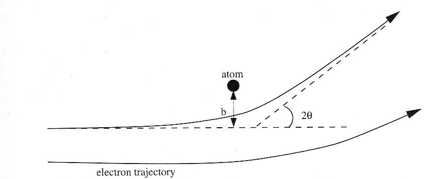
See Atomic Form Factor for details

2.5.4. Calculate Structure Factors#

To extend the single atom view of the atomic form factor $f (θ$ ) to a crystal, we change to the structure factor $F (θ)$ . The structure factor $F (θ)$ is a measure of the amplitude scattered by a unit cell of a crystal structure.

Because $F (θ)$ is an amplitude like $f (θ)$ , it also has dimensions of length.We can define $F (θ)$ as: $ $F_{h k l} (θ) = \sum_{j = 1}^{inf} f_{j} (θ) e^{[- 2 π i (h x_{j} + k y_{j} + l z_{j})]}$ $

F_{h k l} (θ) = \sum_{j = 1}^{inf} f_{j} (θ) e^{[- 2 π i ({\vec{g}}_{h} x_{j} + {\vec{g}}_{k} y_{j} + {\vec{g}}_{l} l z_{j})]}

F_{h k l} (θ) = \sum_{j = 1}^{inf} f_{j} (θ) e^{[- 2 π i ({\vec{g}}_{h k l} \cdot {\vec{r}}_{j})]}

The sum is over all the $i$ atoms in the unit cell (with atomic coordinates ${\vec{r}}_{i} = [x_{i}, y_{i}, z_{i}]$ )

The structure factors $f_{i} (θ)$ are multiplied by a phase factor (the exponential function). The phase factor takes account of the difference in phase between waves scattered from atoms on different but parallel atomic planes with the same Miller indices $(h k l)$ .

The scattering angle $θ$ is the angle between the angle between the incident and scattered electron beams.

Please identify all the variables in line 10 below. Please note that we only do a finite number of hkl

# Calculate Structure Factors

structure_factors = []

base = atoms.positions  # positions in Carthesian coordinates
for j  in range(len(g_hkl)):
    F = 0
    for b in range(len(base)):
        theta = np.linalg.norm(np.dot(g_hkl[j], reciprocal_lattice))  # angle in 1/nm 
        f = ks.feq(atoms[b].symbol, theta) # Atomic form factor for element and momentum change (g vector)
        F += f * np.exp(-2*np.pi*1j*(g_hkl[j]*base[b]).sum())        
    structure_factors.append(F)
F = structure_factors = np.array(structure_factors)

2.5.4.1. All Allowed Reflections#

The structure factor determines whether a reflection is allowed or not.

If the structure factor is zero, the reflection is called forbidden.

# Allowed reflections have a non zero structure factor F (with a  bit of numerical error)
allowed = np.absolute(structure_factors) > 0.001

print(f' Of the evaluated {hkl.shape[0]} Miller indices {allowed.sum()} are allowed. ')

distances = np.linalg.norm(g_hkl, axis = 1)
# We select now all the 
zero = distances == 0.
allowed = np.logical_and(allowed,np.logical_not(zero))

F = F[allowed]
g_hkl = g_hkl[allowed]
hkl = hkl[allowed]
distances = distances[allowed]

 Of the evaluated 2197 Miller indices 387 are allowed.

2.5.4.2. Families of reflections#

reflections with the same length of reciprocal lattice vector are called families

sorted_allowed = np.argsort(distances)

distances = distances[sorted_allowed]
hkl = hkl[sorted_allowed]
F = F[sorted_allowed]

# How many have unique distances and what is their muliplicity

unique, indices  = np.unique(distances, return_index=True)

print(f' Of the {allowed.sum()} allowed Bragg reflections there are {len(unique)} families of reflections.')

 Of the 386 allowed Bragg reflections there are 20 families of reflections.

2.5.4.3. Intensities and Multiplicities#

In a cubic system, the all reflection belonging to one families have the same reciprocal lattice vector and the same probability of scattering.

multiplicitity = np.roll(indices,-1)-indices
intensity = np.absolute(F[indices]**2*multiplicitity)
print('\n index \t     hkl \t 1/d [1/Ang]     d [pm] \t  F \t multip. intensity' )
family = []
for j in range(len(unique)-1):
    i = indices[j]    
    i2 = indices[j+1]   
    family.append(hkl[i+np.argmax(hkl[i:i2].sum(axis=1))])
    print(f'{i:3g}\t {family[j]} \t  {distances[i]:.2f}  \t {1/distances[i]*100:.0f} \t {np.absolute(F[i]):.2f}, \t  {indices[j+1]-indices[j]:3g} \t {intensity[j]:.2f}') 
    # print(f'{i:3g}\t'+ '{'+f'{family[j][0]:.0f} '+f'{family[j][1]:.0f} '+f'{family[j][2]:.0f}' +'}'+f' \t  {distances[i]:.2f}  \t {1/distances[i]*100:.0f} \t {np.absolute(F[i]):.2f}, \t  {indices[j+1]-indices[j]:3g} \t {intensity[j]:.2f}') 
    

 index 	     hkl 	 1/d [1/Ang]     d [pm] 	  F 	 multip. intensity
  0	 [1. 1. 1.] 	  0.32  	 314 	 32.05, 	    8 	 8219.25
  8	 [0. 2. 2.] 	  0.52  	 192 	 43.49, 	   12 	 22694.18
 20	 [1. 3. 1.] 	  0.61  	 164 	 30.02, 	   24 	 21627.29
 44	 [0. 4. 0.] 	  0.74  	 136 	 40.83, 	    6 	 10004.44
 50	 [3. 1. 3.] 	  0.80  	 125 	 28.23, 	   24 	 19122.83
 74	 [4. 2. 2.] 	  0.90  	 111 	 38.48, 	   16 	 23693.10
 90	 [2. 2. 4.] 	  0.90  	 111 	 38.48, 	    8 	 11846.55
 98	 [1. 1. 5.] 	  0.96  	 105 	 26.63, 	    8 	 5674.85
106	 [3. 3. 3.] 	  0.96  	 105 	 26.63, 	   24 	 17024.55
130	 [4. 4. 0.] 	  1.04  	 96 	 36.38, 	   12 	 15880.30
142	 [3. 5. 1.] 	  1.09  	 92 	 25.20, 	   48 	 30493.62
190	 [2. 6. 0.] 	  1.16  	 86 	 34.48, 	   24 	 28539.58
214	 [3. 3. 5.] 	  1.21  	 83 	 23.92, 	   24 	 13726.58
238	 [4. 4. 4.] 	  1.28  	 78 	 32.77, 	    8 	 8590.36
246	 [5. 5. 1.] 	  1.31  	 76 	 22.75, 	   24 	 12416.23
270	 [2. 4. 6.] 	  1.38  	 73 	 31.21, 	   48 	 46748.74
318	 [5. 3. 5.] 	  1.41  	 71 	 21.68, 	   24 	 11279.07
342	 [0. 6. 6.] 	  1.56  	 64 	 28.47, 	   12 	 9728.70
354	 [5. 5. 5.] 	  1.59  	 63 	 19.81, 	    8 	 3138.30

2.5.5. Allowed reflections for Silicon:#

$| F_{h k l} |^{2} = {\begin{cases} (h, k, l all odd \\ (h, | k, l all even & and h + k + l = 4 n \end{cases}$

Check above allowed reflections whether this condition is met for the zero order Laue zone.

Please note that the forbidden and alowed reflections are directly a property of the structure factor.

2.5.6. Diffraction with parallel Illumination#

Polycrystalline Sample	Single Crystalline Sample
ring pattern	spot pattern
depends on $F (θ)$	depends on $F (θ)$

	| depends on excitation error $s$

2.5.7. Ring Pattern#

Ring Pattern:

The profile of a ring diffraction pattern (of a polycrystalline sample) is very close to what a you are used from X-ray diffraction.
The x-axis is directly the magnitude of the $| \vec{g} | = 1 / d$ of a hkl plane set.
The intensity of a Bragg reflection is directly related to the square of the structure factor $I = F^{2} (θ)$
The intensity of a ring is directly related to the multiplicity of the family of planes.

Ring Pattern Problem:

Where is the center of the ring pattern
Integration over all angles (spherical coordinates)
Indexing of pattern is analog to x-ray diffraction.

The Ring Diffraction Pattern are completely defined by the Structure Factor

from matplotlib import patches
fig, ax = plt.subplots()
plt.scatter(0,0);
img = np.zeros((1024,1024))
extent = np.array([-1,1,-1,1])*np.max(unique)
plt.imshow(img, extent = extent)

for radius in unique:   
    circle = patches.Circle((0,0), radius*2, color='yellow', fill= False, alpha = 0.5)#, **kwargs)
    ax.add_artist(circle);
    
plt.xlabel('scattering angle (1/$\AA$)');

2.5.8. Conclusion#

The scattering geometry provides all the tools to determine which reciprocal lattice points are possible and which of them are allowed.

Next we need to transfer out knowledge into a diffraction pattern.