Chapter 4: Spectroscopy

Quantify Spectrum¶

part of

MSE672: Introduction to Transmission Electron Microscopy

by Gerd Duscher, Spring 2026

Microscopy Facilities
Institute of Advanced Materials & Manufacturing
Materials Science & Engineering
The University of Tennessee, Knoxville

Background and methods to analysis and quantification of data acquired with transmission electron microscopes.

First we import the essential libraries¶

All we need here should come with the annaconda or any other package

The xml library will enable us to read the Bruker file.

Cross-section for EDS in Transmission¶

For thin samples such as used in transmission electron microscopy absorption, and fluorescence, can be neglected Chapter 2: Pennycook and Nellist, 2011. If multiple scattering and channelling is avoided the EDS partial scattering cross-section for a single atom of element x is given by Macarthur et al., 2015 and Macarthur et al., 2017:

Where:

• $N_x$: the volumetric number density of the elemental species being detected,

• $t$: the sample thickness (same length unit as volume in N_x),

• $I_x$: is the raw x-ray counts detected from the sample (a.u.),

• $i_0$: is the probe current (A),

• $\tau$ is the exposure time (s),

• $e$ is the electronic charge (C).

A more consistent way would be to relate the cross-section with areal density $n_x$ and to use incident flux $I_0$ like in the case of EELS earlier.

Where:

• $n_x = \rho_x *t$: the areal density of the elemental species being detected,

• $I_0 = i_0*\tau/e$: incident flux: total number of electrons the sample is exposed to during the experiment

Comparison with EELS¶

Above formula is the same as derived for EELS earlier. The difference is that $I_x^{EELS}$ is the number of electrons that scattered inelastically per energy transfer (and momentum transfer).

While $I_x^{EDS}$ is the raw counts of X-rays that originate in the relaxation of excitation from a specific core level of element $x$. This implies that the competing relaxation process of generation of Auger electrons is the same for all elements.

This is a fundamental requirement for quantification of both EDS and Auger spectroscopy.

The relationship between $\sigma_{x}^{EDS}$ and $\sigma_{x}^{EELS}$ is, therfore, a linear one. And we need to determine the efficiency of X-ray detection (not generation) per EDS system, which also has an take-off angle dependence.

However, the linear dependency is not between the EELS and EDS cross section as defined here, but the cross section of the core excitation, as introduced by Egerton. In that approach the inelastic scattering of lower-energy core-losses are approximated together with the background caused by plasmon losses.

Therefore, in the code cell below we need to subtract the background from lower-level excitations from the core-level in question.

Cross-section for EDS¶

Of course we do not need the dependence of the cross section on energy but the sum.

The relevant functions will then be:

Comparison to k-factors to Cliff Lorimer

• k-factors are in weight%

• cross-sections in atom%

The above cross sections are for the excitation of a specific core-level of an atom. The sum of the experimental detected X-ray lines of one family are a fraction of those cross-sections.

Given the large discrepancy of excitation probabilities of the different core-levels, we use the lower-energy cross-sections if possible. Adding up the different families will result in sup-percent change in the total percentage of excitation probabilties.

Varambhia et al. used the linear thickness dependence of the signal to correlate the cross sections of EDS and EELS. This is an excellent way to callibrate the EDS system. And the correlation factor between EELS and EDS should be same for different X-Ray peak families of all elements. The similar method can be used to callibrate the cross section of ADF intensities.

k-Factor for relative composition¶

the k-factor for elements A and B is defined as:

• $Q$ [ionizations/e$^-$ (atoms / cm$^2$)): ionization cross section

• $\omega$ [X-rays/ ionization]: fluorescent yield = number of X-rays generated per ionization

• $A$ [g/moles]: atomic weight

• $a$ relative transition probability (a) of the same series of X-rays ($\alpha\ to\ \beta$)

• $\varepsilon$ detector efficiencies for lines. If we look back to the Ch4_14 and the generation of X-rays, we see that we eliminated the variables of the sample (areal density) , because they are the same.

rewriting above equation we see that:

We do not worry about the units. Since we are fitting all lines we can omit the relative transition probability.

The main uncertainties are: The cross section, and the fluorescent yield.

There are three customary reference elements for the k-factor:

• silicon (semiconductor industrie and literature )

• iron (materials science)

• carbon (ThermoFisher seems to be using that)

Using silicon we need the $k_{ASi}$ factors and

Only for thicker samples we need the density and thickness for absorption corrections.

Atomic-resolution EDS¶

For atomic-resolution studies, an integration of the counts over a Voronoi cell in the EDX map gives a partial cross-section for that column, by analogy with the approach for ADF cross-sections (E et al., 2013). For comparison, the popularly used ζ-factor method defined by (Watanabe et al., 2003) is:

Where

• $I_x$ is the raw x-ray counts,

• ρ is the sample density in kg/m3,

• t is the sample thickness,

• $C_x$ is the weight fraction of element x.

In Eq. (2), the definition of sample density in the zeta-factor approach is in kg/m3 which makes absolute quantification of nanoparticles, in terms of “number of atoms”, cumbersome. Nonetheless, partial cross-section is very similar to the ζ-factor and can be equated to it using Eq. (4). Where M is the molar mass (in kg/mol) and NA is Avogadro’s constant.

Open a EDS spectrum file¶

Here the EDS-STO.emd file in the example_data folder.

Element Finding With pyTEMlib¶

The minimum_number_of_peaks determines how many elements will be found.

Increase from 10 to 11 of that parameter will reveal Nb, a common dopant of SrTiO$_3$

Quantify¶

In the model based approach with want to fit the spectrum with its basic features

These basic features in an EDS spectrum are:

• Background dominated by

  • Bremsstrahlung

  • Detector effciency

• Characteristic Peaks

Fit spectrum¶

Composition Basis¶

Castaing’s first approximation:¶

• $𝐶_i$ = Concentration of element $𝑖$

• $𝐼_𝑖$ = X-ray intensity of element $𝑖$ in the sample

• $𝐼_{𝑃𝑢𝑟𝑒}$ = X-ray intensity of a pure sample of the element

We call the ratio: $\frac{I_i}{I_{Pure}}$ k-ratio

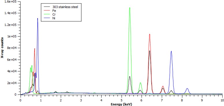
• Stainless to Fe-Ka ratio = 0.745

• Stainless to Cr-Ka ratio = 0.208

• Stainless to Ni-Ka ratio = 0.080

therefore:

• Fe: 70.8 wt%

• Cr: 17.2 wt%

• Ni: 9.1 wt%

Quantify Spectrum¶

first with Bote-Salvat cross section using dictionaries calculated with emtables package.

then with k-factor dictionary

ZAF Correction¶

While the k-ratio is a good starting point, the basic approximation does not take absorption and interaction between the different elements into account. To increase the precision the following corrections are applied:

• Z: Atomic number factor

• A: sample Absorption

• F: Fluorescence

Atomic Number Factor - Z¶

The stopping power is equal to the energy loss of the electron per unit length it travels in the material: $𝑆(𝐸)=−𝑑𝐸/𝑑t$

D.C. Joy, Microsc. Microanal. 7(2001): 159-169

• $E$: electron energy

• $\rho$: density of material

• $Z$: Atomic number

• $A$: atomic weight of material

• $J$: Mean ionizaton potential

The backscatter correction is the relation between how many photons are generated with and without backscattering.

• $R$: backscatter correction

• $Z$: Mean atomic number of sample

• $E_0$: electron energy

• $E_c$: critical ionization energy

Absorption Correction¶

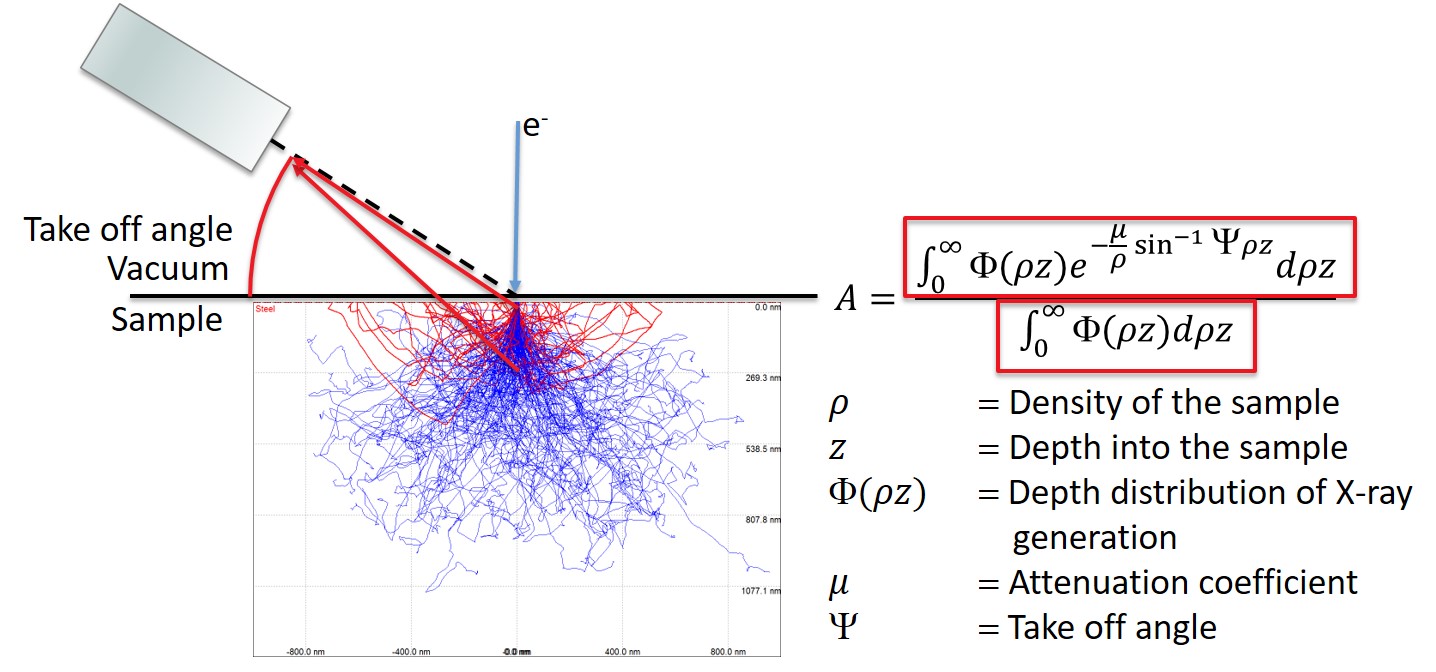
The numerator describes how many X-rays are generated at a given depth and scales the number by the attenuation due to the escape path in the sample.

The denominator is the total number of X-rays generated without attenuation.

This means that A is a normalized value that describes how many of the generated X-rays actually escaped the sample.

Takeoff angle and Absorption¶

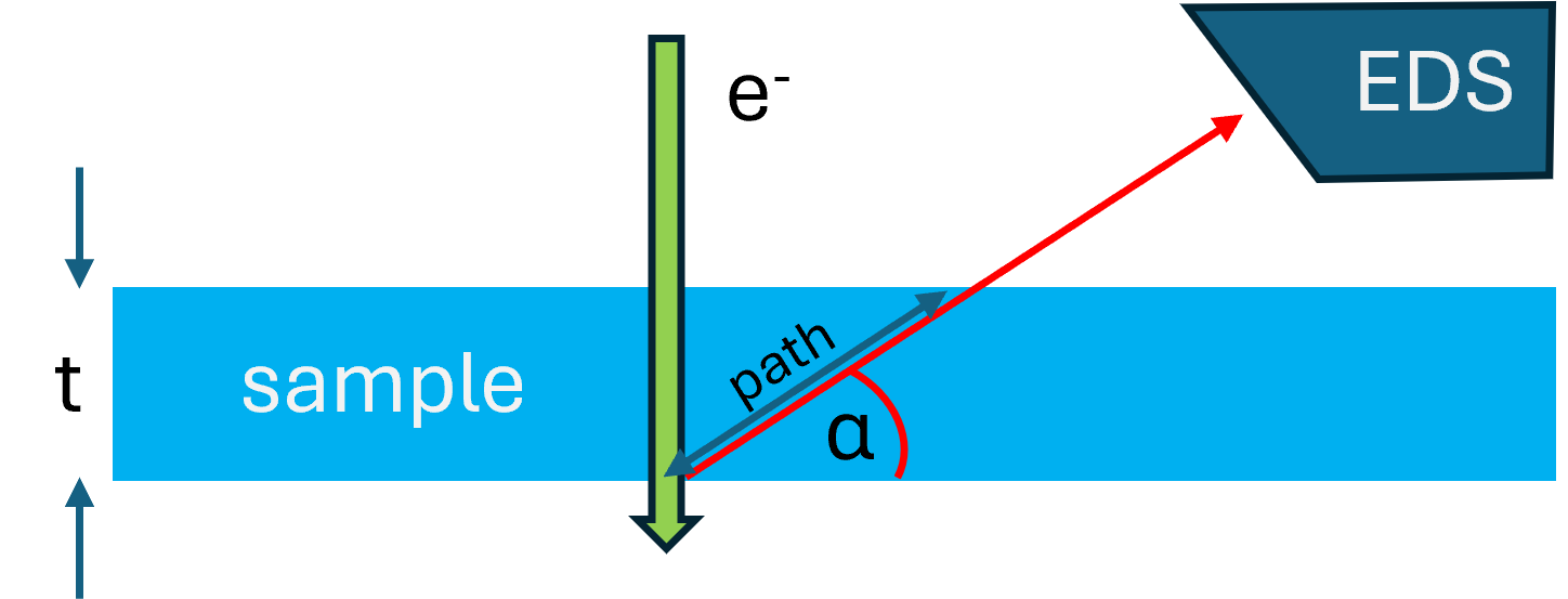
After an X-ray is emitted it may get absorbed by an other atom with a line of lower energy. In NiO the Ni-K X-ray photon can be absobed by the O-K edge and thus the oxygen signal is more prominent than the chemical composition would allow. Therefore, the path-length of the X-rays within the sample to the detector is important With a sample-thickness $t$ and take-off angle $\alpha$, the path-length $p$ in the sample is:

NOTE

Absorption is not important for thin specimens (< ~50nm)

The absorption coefficient is defined as :

with: $\varphi_B(\rho t)$ : depth distribution of Xray production

which is the ratio of the X-ray emission from a layer of element A/B of thickness $\Delta \rho t$ at depth $t$ in the specimen with density $\rho$ to the X-ray emission from an identical, but isolated film.

$\left. \frac{\mu}{\rho} \right]^A_{\rm spec} = \sum_i \left( \left. \frac{C_i\mu}{\rho} \right]^A_{\rm spec} \right)$ : the mass-absorption coefficient of X-rays from element A in the specimen ($C_i$ concentration of element $i$ with $\sum_i C_i =1$)

$\alpha$ : the detector take-off angle.

Note

The sample acts like the detector and will absorbe part of the photons emitted

This absorption is treatd like the detector but the elements depend on the sample

In a TEM we can assume that the film is homogeneous and can set $\varphi_B(\rho t) = 1$

and we get:

For absorption correction, we need to know desnity $\rho$ and thickness $t$ of our specimen.

Absorption with pyTEMlib¶

Please note that this is the only correction needed in TEM

Lower energy lines will be more affected than higher x-ray lines.

At thin sample location (<50nm) absorption is not significant.

Fluorescence Correction¶

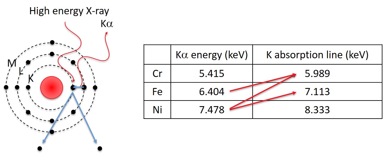
The high energy X-ray can originate from characteristic X-rays from elements with higher energy lines or from the bremsstrahlung. This means that even the element with the highest energy line can have a fluorescence correction.

Using ZAF¶

ZAF assumptions¶

Several assumptions are made either directly or indirectly in the equations used to calculate the composition of a sample.

• The sample is homogenous.

  • The density 𝜌 and the mass attenuation 𝜇/𝜌 is assumed to be constant.

• The sample is flat.

  • 𝑧 is well defined for any given position and no additional absorption takes place after the X-ray reaches the sample surface.

• The sample is infinitely thick as seen by the electron beam.

  • -The energy of the incident electron is deposited in the sample and only secondary and backscatter electrons escape.

Composition Standardless¶

For standard-less analysis the k-ratio is either calculated in the software or based on internal standards.

Following

D.E. Newbury, C.R. Swyt, and R.L. Myklebust, “Standardless” Quantitative Electron Probe Microanalysis with Energy-Dispersive X-ray Spectrometry: Is It Worth the Risk?, Anal. Chem. 1995, 67, 1866-1871

to calculate the mass concentration $C_i$ from the intensity of a line ($I_{ch}$), we use:

• $\omega$ : fluorescence yield

• $N_A$: Avogadro’s number

• $\rho$: density

• $C_i$: mass concentration of element $i$

• $A$:atomic weight

• $R$: backscatter loss

• $Q_i$: ionization cross section

• $dE/ds$: rate of energy loss

• $E_0$: incident beam energy

• $E_c$: excitation energy

• $\epsilon$: EDS efficiency

where: $N_A * \rho * C_i/A$: volume density of element $i$ (atoms per unit volume)

What do we know at this point?

$\omega; N_A; \rho; A; Q_i; E_0; E_c;$ and $\epsilon$

Summary¶

• EDS quantification is not magic and the results will highly depend on sample preparation and correct peak identification.

• Correct quantification with ZAF relies on the sample being:

  • Flat

  • Homogenous

  • Infinitely thick to the electron beam

• Use of standards is not required for good quantification but it will give additional information and increase quality of the results.

• Peak-to-background based ZAF is good for rough samples but requires better spectra than regular ZAF.

• The best way to good EDS results:

  • Good samples

  • Thorough sample preparation

  • Exact SEM Parameters

Back: Detector Response¶

List of Content: Front¶