Chapter 4 Spectroscopy¶

Analyze Spectrum¶

part of

MSE672: Introduction to Transmission Electron Microscopy

Spring 2024

Gerd Duscher	Khalid Hattar
Microscopy Facilities	Tennessee Ion Beam Materials Laboratory
Materials Science & Engineering	Nuclear Engineering
Institute of Advanced Materials & Manufacturing
The University of Tennessee, Knoxville

Background and methods to analysis and quantification of data acquired with transmission electron microscopes.

Load relevant python packages¶

Check Installed Packages¶

import sys
import importlib.metadata
def test_package(package_name):
    """Test if package exists and returns version or -1"""
    try:
        version = importlib.metadata.version(package_name)
    except importlib.metadata.PackageNotFoundError:
        version = '-1'
    return version

if test_package('pyTEMlib') < '0.2024.2.3':
    print('installing pyTEMlib')
    !{sys.executable} -m pip install  --upgrade pyTEMlib -q

print('done')

installing pyTEMlib
done

First we import the essential libraries¶

All we need here should come with the annaconda or any other package

The xml library will enable us to read the Bruker file.

%matplotlib widget
import matplotlib.pyplot as plt
import numpy as np
import sys
import os
if 'google.colab' in sys.modules:
    from google.colab import output
    from google.colab import drive
    output.enable_custom_widget_manager()
    

import xml
from scipy.ndimage import gaussian_filter

import pyTEMlib
# import pyTEMlib.viz as plot
import pyTEMlib.file_tools as ft
import pyTEMlib.eds_tools as eds

# For archiving reasons it is a good idea to print the version numbers out at this point
print('pyTEM version: ',pyTEMlib.__version__)

Symmetry functions of spglib enabled
Using kinematic_scattering library version {_version_ }  by G.Duscher
pyTEM version:  0.2025.07.0

Select File¶

Please note that the above code cell has to be finished before you can open the * open file* dialog.

Test data are in the SEM_example_data folder, plese select EDS.rto file.

datasets = ft.open_file()

chooser = ft.ChooseDataset(datasets)

dataset = chooser.dataset
dataset.plot()

Function to read Bruker files¶

The data and metadata will be in a python dictionary called tags.

import codecs

def get_bruker_dictionary(fname):
    tree =  xml.etree.ElementTree.parse(fname)
    root = tree.getroot()
    spectrum_number = 0
    i=0
    image_count = 0
    o_count = 0
    tags = {}
    for neighbor in root.iter():
        #print(neighbor, neighbor.attrib)
        
        if 'Type' in neighbor.attrib:
            if 'verlay3' in neighbor.attrib['Type'] :
                semImage = neighbor
                #print(neighbor.attrib['Type'])
                if 'Name' in neighbor.attrib:
                    print('\t',neighbor)
                    print('\t',neighbor.attrib['Type'])
                    print('\t',neighbor.attrib['Name'])
                    print('\t',neighbor.find("./ClassInstance[@Type='TRTSpectrumList']"))
            #if 'TRTImageOverlay' in neighbor.attrib['Type'] : 
            if 'TRTCrossOverlayElement'in neighbor.attrib['Type'] :
                if 'Spectrum' in neighbor.attrib['Name']:
                    #print(o_count)
                    o_count+=1
                    if 'overlay' not in tags:
                        tags['overlay']= {}
                    if 'image'+str(image_count) not in tags['overlay']:
                        tags['overlay']['image'+str(image_count)] ={}
                    tags['overlay']['image'+str(image_count)][neighbor.attrib['Name']] ={}

                    over = tags['overlay']['image'+str(image_count)][neighbor.attrib['Name']]


                    for child in neighbor.iter():
                        if 'verlay' in child.tag:
                            #print(child.tag)
                            pos = child.find('./Pos')
                            if pos != None:
                                over['posX'] = int(pos.find('./PosX').text) 
                                over['posY'] = int(pos.find('./PosY').text) 
                #dd = neighbor.find('Top')
                #print('dd',dd)                       
                #print(neighbor.attrib)
            if 'TRTImageData' in neighbor.attrib['Type'] :
                #print('found image ', image_count)
                dd = neighbor.find("./ClassInstance[@Type='TRTCrossOverlayElement']")
                if dd != None:
                    print('found in image')
                image = neighbor
                if 'image' not in tags:
                    tags['image']={}
                tags['image'][image_count]={}
                im = tags['image'][image_count]
                im['width'] = int(image.find('./Width').text)  # in pixels
                im['height'] = int(image.find('./Height').text)  # in pixels
                im['dtype'] = 'u' + image.find('./ItemSize').text  # in bytes ('u1','u2','u4') 
                im['scale_x'] = float(image.find('./XCalibration').text)
                im['scale_y'] = float(image.find('./YCalibration').text)
                im['plane_count'] = int(image.find('./PlaneCount').text)
                im['date'] = str((image.find('./Date').text))
                im['time'] = str((image.find('./Time').text))
                im['data'] = {}
                for j in range( im['plane_count']):
                    #print(i)

                    img = image.find("./Plane" + str(i))
                    raw = codecs.decode((img.find('./Data').text).encode('ascii'),'base64')
                    array1 = np.frombuffer(raw, dtype= im['dtype'])
                    #print(array1.shape)
                    im['data'][str(j)]= np.reshape(array1,(im['height'], im['width']))
                image_count +=1     
            if 'TRTDetectorHeader' == neighbor.attrib['Type'] :
                detector = neighbor
                tags['detector'] = {}
                for child in detector:
                    if child.tag == "WindowLayers":
                        tags['detector']['window']={}
                        for child2 in child:
                            tags['detector']['window'][child2.tag]={}
                            tags['detector']['window'][child2.tag]['Z'] = child2.attrib["Atom"]
                            tags['detector']['window'][child2.tag]['thickness'] = float(child2.attrib["Thickness"])*1e-5  # stupid units
                            if 'RelativeArea' in child2.attrib:
                                tags['detector']['window'][child2.tag]['relative_area'] = float(child2.attrib["RelativeArea"])
                            
                            
                    else:
                        #print(child.tag , child.text)
                        if child.tag != 'ResponseFunction':
                            if child.text !=None:
                                tags['detector'][child.tag]=child.text
                                
                                if child.tag == 'SiDeadLayerThickness':
                                    tags['detector'][child.tag]=float(child.text)*1e-6
                                    
                                if child.tag == 'DetectorThickness':
                                    tags['detector'][child.tag]=float(child.text)*1e-1
                                    
            # ESMA could stand for Electron Scanning Microscope Analysis
            if 'TRTESMAHeader' == neighbor.attrib['Type'] :
                esma = neighbor
                tags['esma'] ={}
                for child in esma:
                    if child.tag in ['PrimaryEnergy', 'ElevationAngle',  'AzimutAngle', 'Magnification',   'WorkingDistance' ]:
                        tags['esma'][child.tag]=float(child.text)

            if 'TRTSpectrum' == neighbor.attrib['Type'] :
                if 'spectrum' not in tags:
                    tags['spectrum'] = {}    
                if 'Name' in neighbor.attrib:
                    spectrum = neighbor

                    TRTHeader = spectrum.find('./TRTHeaderedClass')

                    if TRTHeader != None:
                        hardware_header = TRTHeader.find("./ClassInstance[@Type='TRTSpectrumHardwareHeader']")

                        spectrum_header = spectrum.find("./ClassInstance[@Type='TRTSpectrumHeader']")

                        result_header = spectrum.find("./ClassInstance[@Type='TRTResult']")
                        #print(i, TRTHeader) 
                        tags['spectrum'][spectrum_number] =  {}
                        tags['spectrum'][spectrum_number]['hardware_header'] ={}
                        if hardware_header != None:
                            for child in hardware_header:
                                tags['spectrum'][spectrum_number]['hardware_header'][child.tag]=child.text
                        tags['spectrum'][spectrum_number]['detector_header'] ={}
                        tags['spectrum'][spectrum_number]['spectrum_header'] ={}
                        for child in spectrum_header:
                            tags['spectrum'][spectrum_number]['spectrum_header'][child.tag]=child.text
                        tags['spectrum'][spectrum_number]['results'] = {}
                        for result in result_header:
                            result_tag = {}
                            for child in result:
                                result_tag[child.tag] = child.text
                            if 'Atom' in result_tag:
                                if result_tag['Atom'] not in tags['spectrum'][spectrum_number]['results']:
                                    tags['spectrum'][spectrum_number]['results'][result_tag['Atom'] ] ={}
                                tags['spectrum'][spectrum_number]['results'][result_tag['Atom']].update(result_tag)
                        tags['spectrum'][spectrum_number]['data'] = np.fromstring(spectrum.find('./Channels').text,dtype='Q', sep=",")

                        spectrum_number+=1

                
    return tags

fname = '../example_data/EDS.rto'
tags = get_bruker_dictionary(fname)


    
index = 0


for key in  tags:     
    print(key)
    #for key in  tags[spectrum]:     
        #print('\t',key,tags[spectrum][key])
        
print(tags['detector'].keys())
print(tags['esma'])

image
overlay
spectrum
detector
esma
dict_keys(['TRTKnownHeader', 'Technology', 'Serial', 'Type', 'DetectorThickness', 'SiDeadLayerThickness', 'DetLayers', 'WindowType', 'window', 'CorrectionType', 'ResponseFunctionCount', 'SampleCount', 'SampleOffset', 'PulsePairResTimeCount', 'PileUpMinEnergy', 'PileUpWithBG', 'TailFactor', 'ShelfFactor', 'ShiftFactor', 'ShiftFactor2', 'ShiftData', 'PPRTData'])
{'PrimaryEnergy': 20.0, 'ElevationAngle': 35.0, 'AzimutAngle': 45.0, 'Magnification': 2274.1145, 'WorkingDistance': 8.9591}

import sidpy 
def tags_to_image(tags, key = 0):

    image = tags['image'][key]
    names = ['x', 'y']
    units = 'nm'
    quantity = 'distance'
    dimension_type='spatial'
    to_nm = 1e3

    scale_x = float(image['scale_x']) * to_nm
    scale_y = float(image['scale_y']) * to_nm
    
    dataset = sidpy.Dataset.from_array(image['data']['0'].T)
    dataset.data_type = 'image'
    dataset.units = 'counts'
    dataset.quantity = 'intensity'
    
    dataset.modality = 'SEM'
    dataset.title = 'image'
    dataset.add_provenance('SciFiReader', 'BrukerReader',  version='0', linked_data = 'File: ')

    
    dataset.set_dimension(0, sidpy.Dimension(np.arange(image['data']['0'].shape[1]) * scale_x,
                                                           name=names[0], units=units,
                                                           quantity=quantity,
                                                           dimension_type=dimension_type))
    dataset.set_dimension(1, sidpy.Dimension(np.arange(image['data']['0'].shape[0]) * scale_y,
                                                           name=names[1], units=units,
                                                           quantity=quantity,
                                                           dimension_type=dimension_type))

    dataset.metadata['experiment'] = tags['esma']
    dataset.metadata['overlay'] = tags['overlay']['image1']
    return dataset

dat = tags_to_image(tags)

v = dat.plot()
dat.x.slope
for key, overlay in dat.metadata['overlay'].items():
    plt.gca().scatter ([overlay['posX']*dat.x.slope], [overlay['posY']*dat.y.slope], marker="x", color='r')
    plt.gca().text((overlay['posX']+5)*dat.x.slope, (overlay['posY']-5)*dat.x.slope, key, color='r')

v = dat.plot()

%matplotlib widget
import SciFiReaders
import matplotlib.pylab as plt
fname = '../example_data/EDS.rto'
reader = SciFiReaders.BrukerReader(fname)
datasets = reader.read()
image =  datasets['Channel_000']
v = image.plot()

for key, overlay in image.metadata['overlay'].items():
    plt.gca().scatter ([overlay['pos_x']*image.x.slope], [overlay['pos_y']*image.y.slope], marker="x", color='r')
    plt.gca().text((overlay['pos_x']+5)*image.x.slope, (overlay['pos_y']-5)*image.y.slope, key, color='r')

spectrum1 = datasets['Channel_001']
spectrum2 = datasets['Channel_002']

plt.figure()
plt.plot(spectrum1.energy_scale.values/1000, spectrum1, label='spectrum 1')
plt.plot(spectrum2.energy_scale.values/1000, spectrum2, label='spectrum 2')
plt.gca().set_xlabel('energy [keV]');

def get_spectrum(tags, key=0):
    spectrum = tags['spectrum'][key]
    offset = float(spectrum['spectrum_header']['CalibAbs'])
    scale  = float(spectrum['spectrum_header']['CalibLin'])
    energy_scale = np.arange(len(spectrum1))*scale+offset
    dataset = sidpy.Dataset.from_array(spectrum['data'])
    energy_scale = (np.arange(len(dataset))*scale+offset)*1000
    dataset.units = 'counts'
    dataset.quantity = 'intensity'
    dataset.data_type = 'spectrum'
    
    dataset.modality = 'EDS'
    dataset.title = 'spectrum'
    dataset.set_dimension(0, sidpy.Dimension(energy_scale,
                                             name='energy_scale', units='eV',
                                             quantity='energy',
                                             dimension_type='spectral'))

    dataset.metadata['experiment'] = tags['esma']
    dataset.metadata['EDS'] = {'detector': tags['detector']} 
    dataset.metadata['EDS']['results'] = {}
    for key, result in spectrum['results'].items():
        if 'Name' in result:
            key = result['Name']
            dataset.metadata['EDS']['results'][result['Name']] = result
    
    return dataset

da = get_spectrum(tags, key=0)
da.plot()
da.metadata['EDS']['detector']['window'].keys()

tags['spectrum'][0]['detector_header']

{}

da = get_spectrum(tags['spectrum'][0])
da.plot()

print(tags['spectrum'][0]['results']['6'])

{'Atom': '6', 'XLine': 'K-Serie', 'AtomPercent': '6.061812135E-1', 'MassPercent': '5.374531664E-1', 'NetIntens': '1.121282398E5', 'Background': '6.5E2', 'Sigma': '1.124106061E-1', 'ErrorFlag': '12', 'FCorrection': '1', 'Name': 'C', 'Description': 'C-Ka', 'Line': 'KA', 'Energy': '2.77E-1', 'Width': '9.238120656E-2', 'Counts': '106426', 'NetCounts': '106043'}

tree =  xml.etree.ElementTree.parse(fname)
root = tree.getroot()
i=0
for child in root:
    i+=1
    if i>20:
        break
    if  len(child.attrib) == 0:
        print(child.tag, child.attrib, child.text)

RTHeader {} None

!pip install xmltodict

Collecting xmltodict
  Downloading xmltodict-0.14.2-py2.py3-none-any.whl.metadata (8.0 kB)
Downloading xmltodict-0.14.2-py2.py3-none-any.whl (10.0 kB)
Installing collected packages: xmltodict
Successfully installed xmltodict-0.14.2


depth = 0
my_d = {}
def read_xml(root, my_d):
    for child in root:
        # print(child.tag, child.attrib)
        if hasattr(child, 'attrib'):
            if len(child.attrib) >0:
                my_d[child.tag] = {}
                read_xml(child, my_d[child.tag])
           

read_xml(root, my_d)
my_d

{'ClassInstance': {}}

spectrum1 =tags['spectrum'][0]['data']
spectrum2 =tags['spectrum'][1]['data']
offset = float(tags['spectrum'][0]['spectrum_header']['CalibAbs'])
scale  = float(tags['spectrum'][0]['spectrum_header']['CalibLin'])
energy_scale1 = np.arange(len(spectrum1))*scale+offset
offset = float(tags['spectrum'][1]['spectrum_header']['CalibAbs'])
scale  = float(tags['spectrum'][1]['spectrum_header']['CalibLin'])
energy_scale2 = np.arange(len(spectrum2))*scale+offset
plt.figure()
plt.plot(energy_scale1,spectrum1, label = 'spectrum 1')
plt.plot(energy_scale2,spectrum2, label = 'spectrum 2')
plt.gca().set_xlabel('energy [keV]');

print(tags['overlay'].keys())
print(tags['overlay']['image1'])
#print(tags['3']['hardware_header'])
print(tags['detector'])
print(tags['esma'])
#print(tags['3']['spectrum_header'])

dict_keys(['image1', 'image2'])
{'Spectrum 1': {'posX': 483, 'posY': 504}, 'Spectrum 2': {'posX': 191, 'posY': 277}}
{'TRTKnownHeader': '\n                ', 'Technology': 'SDDpr', 'Serial': '11960', 'Type': 'XFlash 6|30', 'DetectorThickness': 0.045000000000000005, 'SiDeadLayerThickness': 2.9e-08, 'DetLayers': 'eJyzcUkt8UmsTC0qtrMB0wYKjiX5ubZKhsZKCiEZmcnZeanFxbZKpq66xkr6UDWGUDXmKEos9ICKjOCKjKCKTFEUmSGbYwxVYoZbiQlUiQWqErhV+gj3AwCpRT07', 'WindowType': 'slew AP3.3', 'window': {'Layer0': {'Z': '5', 'thickness': 1.3e-07}, 'Layer1': {'Z': '6', 'thickness': 1.45e-06}, 'Layer2': {'Z': '7', 'thickness': 4.5000000000000003e-07}, 'Layer3': {'Z': '8', 'thickness': 8.500000000000001e-07}, 'Layer4': {'Z': '13', 'thickness': 3.5000000000000004e-07}, 'Layer5': {'Z': '14', 'thickness': 0.0038000000000000004, 'relative_area': 0.23}}, 'CorrectionType': '3', 'ResponseFunctionCount': '21', 'SampleCount': '5', 'SampleOffset': '-3', 'PulsePairResTimeCount': '8', 'PileUpMinEnergy': '4.00000006E-1', 'PileUpWithBG': '1', 'TailFactor': '1', 'ShelfFactor': '1', 'ShiftFactor': '3.720000088E-1', 'ShiftFactor2': '-8.500000238E-1', 'ShiftData': '0.069977,0.005798,0.182983,0.007797,0.276978,0.005798,0.554932,0,1.099609,0,3.292969,0.006397,5.888672,0,0,0,0,0,', 'PPRTData': '0.95,2.891959,1.05,2.195911,1.55,1.700256,1.75,1.604574,3.75,1.155987,4.55,0.980248,5.95,1.003,8.05,1.004377,'}
{'PrimaryEnergy': 20.0, 'ElevationAngle': 35.0, 'AzimutAngle': 45.0, 'Magnification': 2274.1145, 'WorkingDistance': 8.9591}

plt.figure(figsize=(10,4))

ax1 = plt.subplot(1,2,1)
ax1.imshow(tags['image']['0']['data']['0'])
for key in tags['overlay']['image1']:
    d = tags['overlay']['image1'][key]
    ax1.scatter ([d['posX']], [d['posY']], marker="x", color='r')
    ax1.text(d['posX']+5, d['posY']-5, key, color='r')

ax2 = plt.subplot(1,2,2)    
plt.plot(energy_scale1,spectrum1, label = 'spectrum 1')
plt.plot(energy_scale2,spectrum2, label = 'spectrum 2')
plt.gca().set_xlabel('energy [keV]')
plt.xlim(0,5)
plt.ylim(0)
plt.tight_layout()
plt.legend();

Find Maximas¶

Of course we can find the maxima with the first derivative

from scipy.interpolate import InterpolatedUnivariateSpline

# Get a function that evaluates the linear spline at any x
f = InterpolatedUnivariateSpline(energy_scale1,spectrum1, k=1)

# Get a function that evaluates the derivative of the linear spline at any x
dfdx = f.derivative()

# Evaluate the derivative dydx at each x location...
dydx = dfdx(energy_scale1)
from scipy.ndimage import gaussian_filter


plt.figure()
plt.plot(energy_scale1,spectrum1, label = 'spectrum 1')

#plt.plot(energy_scale1, dydx)
plt.plot(energy_scale1,gaussian_filter(dydx, sigma=3)/10)
plt.gca().axhline(y=0,color='gray')
plt.gca().set_xlabel('energy [keV]');

Peak Finding¶

We can also use the peak finding routine of the scipy.signal to find all the maxima.

import scipy as sp 
import scipy.signal as sig

start = np.searchsorted(energy_scale1, 0.125)
## we use half the width of the resolution for smearing
width = int(np.ceil(125*1e-3/2 /(energy_scale1[1]-energy_scale1[0])/2)*2+1)
new_spectrum =  sp.signal.savgol_filter(spectrum1[start:], width, 2) ## we use half the width of the resolution for smearing
new_energy_scale = energy_scale1[start:]
major_peaks, _  = sp.signal.find_peaks(new_spectrum, prominence=1000)  
minor_peaks, _  = sp.signal.find_peaks(new_spectrum, prominence=30)  
peaks = major_peaks

spectrum1 = np.array(spectrum1)
plt.figure()
plt.plot(energy_scale1,spectrum1, label = 'spectrum 1')
#plt.plot(energy_scale1,gaussian_filter(spectrum1, sigma=1), label = 'filtered spectrum 1')
plt.plot(new_energy_scale,new_spectrum, label = 'filtered spectrum 1')
plt.scatter( new_energy_scale[minor_peaks], new_spectrum[minor_peaks], color = 'blue')
plt.scatter( new_energy_scale[major_peaks], new_spectrum[major_peaks], color = 'red')

plt.xlim(.126,5);

Peak identification¶

Here we look up all the elemetns and see whether the position of major line (K-L3, K-L2’ or ‘L3-M5’) coincides with a peak position as found above.

Then we plot all the lines of such an element with the appropriate weight.

The positions and the weight are tabulated in the ffast.pkl file introduced in the Characteristic X-Ray peaks notebook

import pickle 
pkl_file = open('data/ffast.pkl', 'rb')
ffast = pickle.load(pkl_file)
pkl_file.close()

plt.figure()
#plt.plot(energy_scale1,spectrum2, label = 'spectrum 1')
#plt.plot(energy_scale1,gaussian_filter(spectrum1, sigma=1), label = 'filtered spectrum 1')
plt.plot(new_energy_scale,new_spectrum, label = 'filtered spectrum 1')
plt.xlim(0.1,4)
plt.ylim(-800)
plt.gca().axhline(y=0,color='gray',  linewidth = 0.5);

out_tags = {}
out_tags['spectra'] = {}

out_tags['spectra'][0] = {}
out_tags['spectra'][0]['data'] = spectrum1
out_tags['spectra'][0]['energy_scale'] = energy_scale1
out_tags['spectra'][0]['energy_scale_start'] = start
out_tags['spectra'][0]['smooth_spectrum'] = new_spectrum
out_tags['spectra'][0]['smooth_energy_scale'] = new_energy_scale

out_tags['spectra'][0]['elements'] ={}


#print(ffast[6])
number_of_elements = 0
for peak in minor_peaks:
    for element in range(1,93):
        if 'K-L3' in ffast[element]['lines']:
            if abs(ffast[element]['lines']['K-L3']['position']- new_energy_scale[peak]*1e3) <10:
                out_tags['spectra'][0]['elements'][number_of_elements] = {}
                out_tags['spectra'][0]['elements'][number_of_elements]['element'] = ffast[element]['element']
                out_tags['spectra'][0]['elements'][number_of_elements]['found_lines'] = 'K-L3'
                out_tags['spectra'][0]['elements'][number_of_elements]['lines'] = ffast[element]['lines']
                out_tags['spectra'][0]['elements'][number_of_elements]['experimental_peak_index'] = peak
                out_tags['spectra'][0]['elements'][number_of_elements]['experimental_peak_energy'] = new_energy_scale[peak]*1e3
                number_of_elements += 1
                plt.plot([ffast[element]['lines']['K-L3']['position']/1000.,ffast[element]['lines']['K-L3']['position']/1000.], [0,new_spectrum[peak]], color = 'red')
                plt.text(new_energy_scale[peak],0, ffast[element]['element']+'\nK-L3', verticalalignment='top')
                for line in ffast[element]['lines']:
                    if 'K' in line:
                        if abs(ffast[element]['lines'][line]['position']-ffast[element]['lines']['K-L3']['position'])> 20:
                            if ffast[element]['lines'][line]['weight']>0.07:
                                #print(element, ffast[element]['lines'][line],new_spectrum[peak]*ffast[element]['lines'][line]['weight'])
                                plt.plot([ffast[element]['lines'][line]['position']/1000.,ffast[element]['lines'][line]['position']/1000.], [0,new_spectrum[peak]*ffast[element]['lines'][line]['weight']], color = 'red')
                                plt.text(ffast[element]['lines'][line]['position']/1000.,0, ffast[element]['element']+'\n'+line, verticalalignment='top')
                            
        elif 'K-L2' in ffast[element]['lines']:
            if abs(ffast[element]['lines']['K-L2']['position']- new_energy_scale[peak]*1e3) <10:
                plt.plot([new_energy_scale[peak],new_energy_scale[peak]], [0,new_spectrum[peak]], color = 'orange')
                plt.text(new_energy_scale[peak],0, ffast[element]['element']+'\nK-L2', verticalalignment='top')
                out_tags['spectra'][0]['elements'][number_of_elements] = {}
                out_tags['spectra'][0]['elements'][number_of_elements]['element'] = ffast[element]['element']
                out_tags['spectra'][0]['elements'][number_of_elements]['found_lines'] = 'K-L2'
                out_tags['spectra'][0]['elements'][number_of_elements]['lines'] = ffast[element]['lines']
                out_tags['spectra'][0]['elements'][number_of_elements]['experimental_peak_index'] = peak
                out_tags['spectra'][0]['elements'][number_of_elements]['experimental_peak_energy'] = new_energy_scale[peak]*1e3
                
                number_of_elements += 1
        if 'L3-M5' in ffast[element]['lines']:
            if abs(ffast[element]['lines']['L3-M5']['position']- new_energy_scale[peak]*1e3) <10:
                pass
                print('found_element', element,ffast[element]['lines']['L3-M5']['position'], new_energy_scale[peak] )
                #plt.scatter( new_energy_scale[peak], new_spectrum[peak], color = 'blue')
                out_tags['spectra'][0]['elements'][number_of_elements] = {}
                out_tags['spectra'][0]['elements'][number_of_elements]['element'] = ffast[element]['element']
                out_tags['spectra'][0]['elements'][number_of_elements]['found_lines'] = 'L3-M5'
                out_tags['spectra'][0]['elements'][number_of_elements]['lines'] = ffast[element]['lines']
                out_tags['spectra'][0]['elements'][number_of_elements]['experimental_peak_index'] = peak
                out_tags['spectra'][0]['elements'][number_of_elements]['experimental_peak_energy'] = new_energy_scale[peak]*1e3
                
                number_of_elements += 1
for element in out_tags['spectra'][0]['elements']:                
    print(out_tags['spectra'][0]['elements'][element]['element'],out_tags['spectra'][0]['elements'][element]['found_lines'])

print(out_tags['spectra'][0]['elements'][0])#['K-L2']['weight'] = 0.5
#del out_tags['spectra'][0]['elements'][7]
for ele in out_tags['spectra'][0]['elements']:
    print(out_tags['spectra'][0]['elements'][ele]['element'])

{'element': 'C', 'found_lines': 'K-L2', 'lines': {'K-L2': {'weight': 0.5, 'position': 277.40000000000003}}, 'experimental_peak_index': 30, 'experimental_peak_energy': 277.577755}
C
O
Mg
Al
P
S
K
Sb

Plotting Gaussians in the Peaks¶

Please note the different width (FWHM). Here I guessed the peak width for two peaks.

def gaussian(enrgy_scale, mu, FWHM):
    sig = FWHM/2/np.sqrt(2*np.log(2))
    return np.exp(-np.power(enrgy_scale - mu, 2.) / (2 * np.power(sig, 2.)))

C_peak = gaussian(new_energy_scale, .275, .068)
P_peak = gaussian(new_energy_scale, 2.019, .095)
plt.figure()

plt.plot(new_energy_scale,new_spectrum, label = 'spectrum')
plt.plot(new_energy_scale,C_peak*8233, label = 'C peak')
plt.plot(new_energy_scale,P_peak*8000, label = 'P peaks', color = 'red')
plt.xlim(.1,3)
plt.legend()

Origin of Line Width¶

Electron hole pairs are created with a standard deviation corresponding to the quantum mechanical shot-noise (Poisson statistic). The distribution is then a Gaussian with the width of the standard deviation $\sigma$ .

For the Mn K-L2,3 peak< this width would be 40 electron hole pairs. The full width at half maximum (FWHM) of the Mn K-L2,3 edge would then be (FWHM of Gaussian is 2.35 * 𝜎) about 106 eV a major component of the observed 125 eV in good EDS systems.

Line Width Estimate¶

Fiori and Newbury 1978 From a reference peak at $E_{ref}$ and the measured FWHM of the peak $FWHM_{ref}$ in eV, we can estimate the peak width of the other peaks

FWHM = \sqrt{2.5 \times (E-E_{ref}) + FWHM_{ref}^2 }

(1)

Gernerally we use the Mn K-L2,3 peak $E_{ref}$ = 5895 eV as a reference. In our spectrometer we got for the setup above: $FWHM_{ref} = 136$ eV

E_ref = 5895.0
FWHM_ref = 136 #eV
E= 275 
def getFWHM(E):
    return np.sqrt(2.5*(E-E_ref)+FWHM_ref**2)

print(getFWHM(E))

66.6783323126786

Using that we get for all peaks in the low energy region:

def getPeak(E, energy_scale):
    E_ref = 5895.0
    FWHM_ref = 136 #eV
    FWHM  = np.sqrt(2.5*(E*1e3-E_ref)+FWHM_ref**2)*1e-3
    return gaussian(energy_scale, E, FWHM)
    
E= .275 
C_peak = getPeak(E,new_energy_scale)
E = 2.019
P_peak = getPeak(E,new_energy_scale)
E = 1.258
Al_peak = getPeak(E,new_energy_scale)
E = 0.528
O_peak = getPeak(E,new_energy_scale)
plt.figure()

plt.plot(new_energy_scale,new_spectrum, label = 'filtered spectrum 1')
plt.plot(new_energy_scale,C_peak*8233, label = 'filtered spectrum 1')
plt.plot(new_energy_scale,P_peak*8000, label = 'filtered spectrum 1')
plt.plot(new_energy_scale,Al_peak*4600, label = 'filtered spectrum 1')

plt.plot(new_energy_scale,O_peak*4600, label = 'filtered spectrum 1')
plt.xlim(.1,3)

Detector Efficiency¶

from scipy.interpolate import interp1d
import scipy.constants as const


## layer thicknesses of commen materials in EDS detectors in m
nickelLayer = 0.* 1e-9 # in m
alLayer = 30 *1e-9    # in m
C_window = 2 *1e-6    # in m
goldLayer = 0.* 1e-9   # in m
deadLayer = 100 *1e-9  # in m
detector_thickness = 45 * 1e-3  # in m

area = 30 * 1e-6 #in m2
oo4pi = 1.0 / (4.0 * np.pi)

#We make a linear energy scale 
energy_scale = np.linspace(.1,60,2000)

## interpolate mass absorption coefficient to our energy scale
lin = interp1d(ffast[14]['E']/1000.,ffast[14]['photoabsorption'],kind='linear') 
mu_Si = lin(energy_scale) * ffast[14]['nominal_density']*100. #1/cm -> 1/m

## interpolate mass absorption coefficient to our energy scale
lin = interp1d(ffast[13]['E']/1000.,ffast[13]['photoabsorption'],kind='linear') 
mu_Al = lin(energy_scale) * ffast[13]['nominal_density'] *100. #1/cm -> 1/m

lin = interp1d(ffast[6]['E']/1000.,ffast[6]['photoabsorption'],kind='linear') 
mu_C = lin(energy_scale) * ffast[6]['nominal_density'] *100. #1/cm -> 1/m
 
detector_Efficiency1 = np.exp(-mu_C * C_window) * np.exp(-mu_Al * alLayer)* np.exp(-mu_Si * deadLayer) 
detector_Efficiency2 = (1.0 - np.exp(-mu_Si * detector_thickness))# * oo4pi;
detector_Efficiency =detector_Efficiency1 * detector_Efficiency2#* oo4pi;

plt.figure()
plt.plot(energy_scale, detector_Efficiency*100, label = 'total absorption')
plt.plot(energy_scale, detector_Efficiency1*100, label = 'detector absorption')
plt.plot(energy_scale, detector_Efficiency2*100, label= 'detector efficiency')
plt.gca().set_xlabel('energy [keV]');
plt.gca().set_ylabel('efficiency [%]') 
plt.legend();
energy_scale = new_energy_scale

Detector Parameters from file¶

print(tags['detector']['window'])
print(tags['detector'].keys())
print(f"{float(tags['detector']['SiDeadLayerThickness'])*1e-6:.3g}")
print(f"{float(tags['detector']['DetectorThickness'])/10:.3f}")
for key in tags['detector']['window']:
    print(f"{tags['detector']['window'][key]['Z']}, {tags['detector']['window'][key]['thickness']*1e-6:.2g}")

{'Layer0': {'Z': '5', 'thickness': 1.3e-07}, 'Layer1': {'Z': '6', 'thickness': 1.45e-06}, 'Layer2': {'Z': '7', 'thickness': 4.5000000000000003e-07}, 'Layer3': {'Z': '8', 'thickness': 8.500000000000001e-07}, 'Layer4': {'Z': '13', 'thickness': 3.5000000000000004e-07}, 'Layer5': {'Z': '14', 'thickness': 0.0038000000000000004, 'relative_area': 0.23}}
dict_keys(['TRTKnownHeader', 'Technology', 'Serial', 'Type', 'DetectorThickness', 'SiDeadLayerThickness', 'DetLayers', 'WindowType', 'window', 'CorrectionType', 'ResponseFunctionCount', 'SampleCount', 'SampleOffset', 'PulsePairResTimeCount', 'PileUpMinEnergy', 'PileUpWithBG', 'TailFactor', 'ShelfFactor', 'ShiftFactor', 'ShiftFactor2', 'ShiftData', 'PPRTData'])
2.9e-14
0.005
5, 1.3e-13
6, 1.5e-12
7, 4.5e-13
8, 8.5e-13
13, 3.5e-13
14, 3.8e-09

Comparison to generic efficiency¶

from scipy.interpolate import interp1d
import scipy.constants as const

def detector_efficiency(tags, energy_scale):
    detector_Efficiency1 = np.ones(len(energy_scale))
    for key in tags['detector']['window']:
        Z = int(tags['detector']['window'][key]['Z'])
        if Z < 14:
            t = tags['detector']['window'][key]['thickness']

            ## interpolate mass absorption coefficient to our energy scale
            lin = interp1d(ffast[Z]['E']/1000.,ffast[Z]['photoabsorption'],kind='linear') 
            mu = lin(energy_scale) * ffast[Z]['nominal_density']*100. #1/cm -> 1/m
            detector_Efficiency1 = detector_Efficiency1 * np.exp(-mu * t)
            print(Z,t)
        
    t = float(tags['detector']['SiDeadLayerThickness'])*1e-6
    print(t)
    t = .30*1e-7
    print(t)
    lin = interp1d(ffast[14]['E']/1000.,ffast[14]['photoabsorption'],kind='linear') 
    mu = lin(energy_scale) * ffast[14]['nominal_density']*100. #1/cm -> 1/m
    detector_Efficiency1 = detector_Efficiency1 * np.exp(-mu * t)
    detector_thickness = float(tags['detector']['DetectorThickness'])*1e-1
    ## interpolate mass absorption coefficient to our energy scale
    mu_Si = lin(energy_scale) * ffast[14]['nominal_density']*100. #1/cm -> 1/m
    print(detector_thickness)
    
    detector_Efficiency2 = (1.0 - np.exp(-mu * detector_thickness))# * oo4pi;

    
    return detector_Efficiency1*detector_Efficiency2
de = detector_efficiency(tags, energy_scale)    
## layer thicknesses of commen materials in EDS detectors in m
nickelLayer = 0.* 1e-9 # in m
alLayer = 30 *1e-9    # in m
C_window = 2 *1e-6    # in m
goldLayer = 0.* 1e-9   # in m
deadLayer = 100 *1e-9  # in m
detector_thickness = 45 * 1e-3  # in m
print(detector_thickness)
area = 30 * 1e-6 #in m2
oo4pi = 1.0 / (4.0 * np.pi)

#We make a linear energy scale 
energy_scale = new_energy_scale


## interpolate mass absorption coefficient to our energy scale
lin = interp1d(ffast[14]['E']/1000.,ffast[14]['photoabsorption'],kind='linear') 
mu_Si = lin(energy_scale) * ffast[14]['nominal_density']*100. #1/cm -> 1/m

## interpolate mass absorption coefficient to our energy scale
lin = interp1d(ffast[13]['E']/1000.,ffast[13]['photoabsorption'],kind='linear') 
mu_Al = lin(energy_scale) * ffast[13]['nominal_density'] *100. #1/cm -> 1/m

lin = interp1d(ffast[6]['E']/1000.,ffast[6]['photoabsorption'],kind='linear') 
mu_C = lin(energy_scale) * ffast[6]['nominal_density'] *100. #1/cm -> 1/m
 
detector_Efficiency1 = np.exp(-mu_C * C_window) * np.exp(-mu_Al * alLayer)#* np.exp(-mu_Si * deadLayer) 
detector_Efficiency2 = (1.0 - np.exp(-mu_Si * detector_thickness))# * oo4pi;
detector_Efficiency =detector_Efficiency1 * detector_Efficiency2#* oo4pi;

plt.figure()
plt.plot(energy_scale*1000, detector_Efficiency , label = 'generic')
plt.plot(energy_scale*1000, de, label = 'UTK detector')
#plt.plot(energy_scale*1000, de* np.exp(-mu_Si * deadLayer) )
#plt.plot(energy_scale*1000, de* np.exp(-mu_Si * deadLayer) * detector_Efficiency2 )
plt.legend();
plt.xlim(0,9000);

Plotting background and lines¶

Peaks = []
elements_peaks = []
intensities = []
for element in out_tags['spectra'][0]['elements']:
    el_dict = out_tags['spectra'][0]['elements'][element]
    
    position = el_dict['lines'][el_dict['found_lines']]['position']
    weight = 0
    for line in el_dict['lines']:
        if abs(position - el_dict['lines'][line]['position'])<20:
            weight += el_dict['lines'][line]['weight']
    index = np.searchsorted(new_energy_scale,el_dict['lines'][el_dict['found_lines']]['position']/1000.)  
    intensity = new_spectrum[index]/weight
    added_peaks = np.zeros(len(new_energy_scale))
    for line in el_dict['lines']: 
        if line[0] == el_dict['found_lines'][0]:
            if el_dict['lines'][line]['weight']> 0.01:
                p = getPeak(el_dict['lines'][line]['position']/1000.,new_energy_scale)*el_dict['lines'][line]['weight']
                Peaks.append(p)
                added_peaks = added_peaks + p 
    elements_peaks.append(added_peaks)        
    intensities.append(intensity)
    
plt.figure()
plt.plot(new_energy_scale,new_spectrum, label = 'filtered spectrum 1')
#plt.plot(new_energy_scale,new_spectrum, label = 'filtered spectrum 1',color='red')
for i in range(len(elements_peaks)):
    plt.plot(new_energy_scale,elements_peaks[i]*intensities[i], label = f'Peak{i}')
    pass
peaks = np.array(Peaks)
plt.plot(new_energy_scale,peaks.sum(axis=0), label = f'Peaks', color = 'blue')
print(peaks.shape)
#plt.xlim(0,5)    
offset = float(tags[0]['spectrum_header']['CalibAbs'])
scale  = float(tags[0]['spectrum_header']['CalibLin'])
energy_scale1 = np.arange(len(spectrum1))*scale+offset
p = [1, 37, .3, offset, scale]
E_0= 20
E = new_energy_scale
N = detector_Efficiency * (p[0] + p[1]*(E_0-E)/E + p[2]*(E_0-E)**2/E)
N = de * (p[0] + p[1]*(E_0-E)/E + p[2]*(E_0-E)**2/E)

pp = p[0:5].copy()
for i in range(len(elements_peaks)):
    pp.append(intensities[i])

plt.plot(new_energy_scale,N, color= 'orange')

plt.xlim(0,4)

detector_Efficiency = de

detector_Efficiency.shape

(2000,)

As a function¶

def model(p,energy_scale):
    E = energy_scale
    
    spectrum = detector_Efficiency * (p[0] + p[1]*(E_0-E)/E + p[2]*(E_0-E)**2/E)
    
    for i in range(5,len(p)):
        spectrum = spectrum+elements_peaks[i-5]*abs(p[i])
    return spectrum
spectrum3 = model(pp[:-1],new_energy_scale)

plt.figure()

plt.plot(new_energy_scale,new_spectrum, label = 'filtered spectrum 1',color='red')
plt.plot(new_energy_scale, spectrum3)
plt.xlim(0,4)

Fitting above function to spectrum¶


from scipy.optimize import leastsq 

## background fitting 
def specfit(p, y, x):
    err = y - model(p,x)
    return err

p, lsq = leastsq(specfit, pp[:-1], args=(new_spectrum, new_energy_scale), maxfev=2000)

print( f'element\t end   \t   start ')
for i, element in enumerate(out_tags['spectra'][0]['elements']):
    if i<len(p)-5:
        el_dict = out_tags['spectra'][0]['elements'][element]
        print(f"{el_dict['element']:2s}: \t  {abs(p[i+5]):6.2f} \t  {pp[i+5]:.2f}")
#print(p,pp)

element	 end   	   start 
C : 	  16487.64 	  16444.49
O : 	  3267.00 	  3274.63
Mg: 	  2831.85 	  3127.80
Al: 	   84.40 	  334.63
P : 	  5267.50 	  5499.66
S : 	   82.35 	  234.96
K : 	  2526.57 	  2693.25

spectrum3 = model(p,new_energy_scale)

plt.figure()

plt.plot(new_energy_scale,new_spectrum, label = 'filtered spectrum 1',color='red')
plt.plot(new_energy_scale, spectrum3)
plt.plot(new_energy_scale, new_spectrum-spectrum3)
plt.gca().axhline(y=0,color='gray');

plt.xlim(0,4);

Energy Scale¶

What happened?

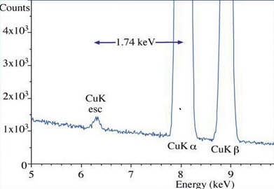
Detector Artifacts¶

Si Escape peak¶

The 1s state of a Si atom in the detector crystal is excited but then instead of being further detected by absoption a A!!uger electron leaves the crystal. The electron hole pairs of this event are missing and a lower energy is recorded.

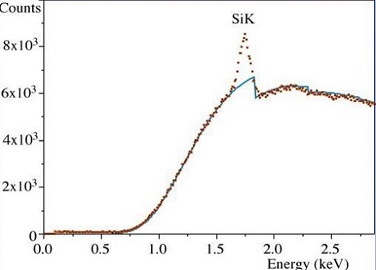
Detector Silicon Peak¶

Internal fluorescence peak

Sum Peak¶

Two photons are detected at the same time. This signal is suppressed by most acquistion systems, but a few are still slipping through. A peak apears at the energy of the sum of two strong peaks.

Composition¶

Following

D.E. Newbury, C.R. Swyt, and R.L. Myklebust, “Standardless” Quantitative Electron Probe Microanalysis with Energy-Dispersive X-ray Spectrometry: Is It Worth the Risk?, Anal. Chem. 1995, 67, 1866-1871

to calculate the mass concentration $C_i$ from the intensity of a line ( $I_{ch}$ ), we use:

I_{ch} = \epsilon (\omega N_A \rho C_i / A) R \int _{E_c}^{E_0} \frac{Q_i}{dE/ds}dE

(2)

$\omega$ : fluorescence yield
$N_A$ : Avogadro’s number
$\rho$ : density
$C_i$ : mass concentration of element $i$
$A$ :atomic weight
$R$ : backscatter loss
$Q_i$ : ionization cross sectiond
$E/ds$ : rate of energy loss
$E_0$ : incident beam energy
$E_c$ : excitation energy
$\epsilon$ : EDS efficiency

where: $N_A * \rho * C_i/A$ : volume density of element $i$ (atoms per unit volume)

What do we know at this point?

$\omega; N_A; \rho; A; Q_i; E_0; E_c; and \epsilon$

def BrowningEmpiricalCrossSection(elm , energy):
    """ * Computes the elastic scattering cross section for electrons of energy between
     * 0.1 and 30 keV for the specified element target. The algorithm comes from<br>
     * Browning R, Li TZ, Chui B, Ye J, Pease FW, Czyzewski Z &amp; Joy D; J Appl
     * Phys 76 (4) 15-Aug-1994 2016-2022

     * The implementation is designed to be similar to the implementation found in
     * MONSEL.
     * Copyright: Pursuant to title 17 Section 105 of the United States Code this
     * software is not subject to copyright protection and is in the public domain
     * Company: National Institute of Standards and Technology
     * @author Nicholas W. M. Ritchie
     * @version 1.0

     */
     Modified by Gerd Duscher, UTK
    """

    #/**
    #* totalCrossSection - Computes the total cross section for an electron of
    #* the specified energy.
    #* 
    # @param energy double - In keV
    # @return double - in square meters
    #*/
    e = energy  #in keV
    re = np.sqrt(e);
    return (3.0e-22 * elm**1.7) / (e + (0.005 * elm**1.7 * re) + ((0.0007 * elm**2) / re));

print(BrowningEmpiricalCrossSection(6,277)*1e18, r'nm^2')

---------------------------------------------------------------------------
NameError                                 Traceback (most recent call last)
Cell In[3], line 1
----> 1 print(BrowningEmpiricalCrossSection(6,277)*1e18, r'nm^2')

Cell In[2], line 27, in BrowningEmpiricalCrossSection(elm, energy)
     19 #/**
     20 #* totalCrossSection - Computes the total cross section for an electron of
     21 #* the specified energy.
   (...)     24 # @return double - in square meters
     25 #*/
     26 e = energy  #in keV
---> 27 re = np.sqrt(e);
     28 return (3.0e-22 * elm**1.7) / (e + (0.005 * elm**1.7 * re) + ((0.0007 * elm**2) / re))

NameError: name 'np' is not defined

Back: Detector Response
Chapter 4: Spectroscopy
List of Content: Front

References¶

Newbury, D. E., Swyt, C. R., & Myklebust, R. L. (1995). “Standardless” Quantitative Electron Probe Microanalysis with Energy-Dispersive X-ray Spectrometry: Is It Worth the Risk? Analytical Chemistry, 67(11), 1866–1871. 10.1021/ac00107a017

Foreword (ReadME)

Chapter 4 Spectroscopy

Foreword (ReadME)

Chapter 4 Spectroscopy

Chapter 4 Spectroscopy

Chapter 4 Spectroscopy¶

Analyze Spectrum¶

Load relevant python packages¶

Check Installed Packages¶

First we import the essential libraries¶

Select File¶

Function to read Bruker files¶

Find Maximas¶

Peak Finding¶

Peak identification¶

Plotting Gaussians in the Peaks¶

Origin of Line Width¶

Line Width Estimate¶

Detector Efficiency¶

Detector Parameters from file¶

Comparison to generic efficiency¶

Plotting background and lines¶

As a function¶

Fitting above function to spectrum¶

Energy Scale¶

Detector Artifacts¶

Si Escape peak¶

Detector Silicon Peak¶

Sum Peak¶

Composition¶

Navigation¶